3. Simulation Performance

This section provides tips for how to implement numerically efficient models and for how to debug models.

All Modelica simulation environments have debugging and profiling capabilities that give insight into where computing time is spent and how to speed up simulations. The use of these features varies among the different Modelica tools. We recommend users read the documentation of their respective simulation environment, take opportunity of training that is offered on request by many tool providers, and contact their support for tool related questions.

3.1. Unstable control loops

Most solvers in Modelica tools adapt the time step during the simulation in order to accurately resolve the dynamics of the model. If feedback control loops are unstable, then trajectories can have high frequency oscillations, just as in a real HVAC system. The solver is then required to simulate with small time steps, which increases the simulation time.

In large models, to detect which control loop is unstable, it can be helpful to log which state variables dominate the integration error or the integrator time step control. This usually points to the control loop that is unstable. There are various methods for tuning a controller, and the documentation of Buildings.Controls.OBC.CDL.Reals.PIDWithReset outlines one approach for tuning the gains of a PI-controller.

3.2. Control input signal of equipment

Most equipment models that take a real-valued control signals as an input, such as flow machines (fans and pumps), have a boolean parameter filteredSpeed, and all actuators have a boolean parameter filteredOpening. If set to true, which is the default setting, then the control input signal is sent to a 2nd order low pass filter that changes a step signal to a smooth signal. This typically improves the robustness of the simulation.

To see the effect of the filter, consider the model below in which fanS is configured with filteredSpeed=false, and fanC is configured with filteredSpeed=true. Both fans are connected to a step input signal. The configuration of fanS causes the fan speed to instantly change from 0 to 1. In large system models, this can lead to high computing time or to convergence problems. The fanC avoids this problem because the speed of the fan varies continuously, thereby making it easier for the solver to compute a solution. In this model, we set the parameter raiseTime=30 seconds.

Fig. 3.1 Schematic diagram of fans that are configured with filteredSpeed=false (fanS) and filteredSpeed=true (fanC).

Fig. 3.2 Mass flow rate of the two fans for a step input signal at 0 seconds.

For fans and pumps, the dynamics introduced by the filter can be thought of as approximating the rotational inertia of the fan rotor and the inertia of the fluid in the duct or piping network. The default value is raiseTime=30 seconds.

For actuators, the raise time approximates the travel time of the valve lift. The default value is raiseTime=120 seconds.

Note

When changing filteredSpeed (or filteredOpening), or when changing the value of raiseTime, the dynamic response of the closed loop control changes. Therefore, control gains may need to be retuned to ensure satisfactory closed loop control performance.

For further information, see the User’s Guide of the flow machine package, and the User’s Guide of the actuator package.

3.3. Fluid flow systems

3.3.1. Breaking algebraic loops

In fluid flow systems, flow junctions where mass flow rates separate and mix can couple non-linear systems of equations. This leads to larger systems of coupled equations that need to be solved, which often causes larger computing time and can sometimes cause convergence problems. To decouple these systems of equations, in the model of a flow junction (Buildings.Fluid.FixedResistances.Junction), or in models for fans or pumps (such as the model Buildings.Fluid.Movers.SpeedControlled_y), the parameter dynamicBalance can be set to true. This adds a control volume at the fluid junction that can decouple the system of equations.

3.3.2. Reducing nonlinear equations of serially connected flow resistances

In fluid flow systems, if multiple components are connected in series, then computing the pressure drop due to flow friction in the individual components can lead to coupled nonlinear systems of equations. While this is no problem for small models, the iterative solution can lead to higher computing time, particularly in large models where other equations may be part of the residual function.

For illustration, consider the simple system shown below in which the flow resistances res1 and res2 compute the mass flow rate as \(\dot m = k \, \sqrt{\Delta p}\) if the parameter from_dp is set to true, or otherwise compute the pressure drop between their inlet and outlet as \(\Delta p = (\dot m / k)^2\). (Both formulations are implemented using regularization near zero.)

Fig. 3.3 Schematic diagram of two flow resistances in series that connect a source and a volume.

Depending on the configuration of the individual component models, simulating this system model may require the iterative solution of a nonlinear equation to compute the mass flow rate or the pressure drop. To avoid a nonlinear equation, use any of the measures below.

• Set the parameter res2(dp_nominal=0), and add the pressure drop to the parameter dp_nominal of the model res1. This will eliminate the equation that computes the flow friction in res2, thereby avoiding a nonlinear equation. The same applies if there are multiple components in series, such as a pre-heat coil, a heating coil and a cooling coil.

• Set from_dp=false in all components, which is the default setting. This will cause Modelica to use a function that computes the pressure drop as a function of the mass flow rate. Therefore, a code translator is likely to generate an equation that solves for the mass flow rate, and it then uses the mass flow rate to compute the pressure drop of the components that are connected in series.

Control valves also allow lumping the pressure drop into the model of the valve. Consider the situation where a fixed flow resistance is in series with a control valve as shown below.

Fig. 3.4 Schematic diagram of a fixed flow resistance and a valve in series that connect a source and a volume.

Suppose the parameters are

Buildings.Fluid.FixedResistances.PressureDrop res(
  redeclare package Medium = Medium,
  m_flow_nominal=0.2,
  dp_nominal=10000);

Buildings.Fluid.Actuators.Valves.TwoWayLinear val(
  redeclare package Medium = Medium,
  m_flow_nominal=0.2,
  dpValve_nominal=5000);

To avoid a nonlinear equation, the flow resistance could be deleted as shown below.

Fig. 3.5 Schematic diagram of a valve that connects a source and a volume.

If the valve is configured as

Buildings.Fluid.Actuators.Valves.TwoWayLinear val(
  redeclare package Medium = Medium,
  m_flow_nominal=0.2,
  dpValve_nominal=5000,
  dpFixed_nominal=10000);

then the valve will compute the composite flow coefficient \(\bar k\) as

\[\bar k = \frac{1}{\sqrt{1/k_v(y) + 1/k_f}}\]

where \(k_v(y) = \dot m(y)/\sqrt{\Delta p}\) is the flow coefficient of the valve at the lift \(y\), and \(k_f\) is equal to the ratio m_flow_nominal/sqrt(dpFixed_nominal). The valve model then computes the pressure drop using \(\bar k\) and the same equations as described above for the fixed resistances. Thus, the composite model has the same valve authority and mass flow rate, but a nonlinear equation can be avoided.

For more details, see the User’s Guide of the actuator package.

3.3.3. Prescribed mass flow rate

For some system models, the mass flow rate can be prescribed by using an idealized pump or fan (model Buildings.Fluid.Movers.FlowControlled_m_flow) or a source element that outputs the required mass flow rate (such as the model Buildings.Fluid.Sources.MassFlowSource_T). Using these models avoids having to compute the intersection of the fan curve and the flow resistance. In some situations, this can lead to faster and more robust simulation.

Warning

If you prescribe the mass flow rate, make sure the pump (or fan) does not work agains a closed valve (or damper). Otherwise, it will force the flow through the component, which leads to very large pressure drops.

3.3.4. Avoiding events

In Modelica, the time integration is halted whenever a Real elementary operation such as \(x>y\), where \(x\) and \(y\) are variables of type Real, changes its value. In this situation, an event occurs and the solver determines a small interval in time in which the relation changes its value. This can increase computing time. An example where such an event occurs is the following relation that computes the enthalpy of the medium that streams through port_a as

if port_a.m_flow > 0 then
  h_a = inStream(port_a.h_outflow);
else
  h_a = port_a.h_outflow;
end if;

or, equivalently,

h_a = if port_a.m_flow > 0 then inStream(port_a.h_outflow) else port_a.h_outflow;

When simulating a model that contains such code, a time integrator will iterate to find the time instant where port_a.m_flow crosses zero. If the modeling assumptions allow approximating this equation in a neighborhood around port_a.m_flow=0, then replacing this equation with an approximation that does not require an event iteration can reduce computing time. For example, the above equation could be approximated as

T_a = Modelica.Fluid.Utilities.regStep(
  port_a.m_flow, inStream(port_a.h_outflow), port_a.h_outflow,
  m_flow_nominal*1E-4);

where m_flow_nominal is a parameter that is set to a value that is close to the mass flow rate that the model has at full load. If the magnitude of the flow rate is larger than 1E-4 times the typical flow rate, the approximate equation is the same as the exact equation, and below that value, an approximation is used. However, for such small flow rates, not much energy is transported and hence the error introduced by the approximation is generally negligible.

In some cases, adding dynamics to the model can further improve the computing time, because the return value of the function Modelica.Fluid.Utilities.regStep() above can change abruptly if its argument port_a.m_flow oscillates in the range of +/- 1E-4*m_flow_nominal, for example due to numerical noise. Adding dynamics may be achieved using a formulation such as

hMed = Modelica.Fluid.Utilities.regStep(
  port_a.m_flow, inStream(port_a.h_outflow), port_a.h_outflow,
  m_flow_nominal*1E-4);
der(h)=(hMed-h)/tau;

where tau>0 is a time constant. See, for example, Buildings.Fluid.Sensors.SpecificEnthalpyTwoPort for a robust implementation.

Note

In the package Buildings.Utilities.Math the functions and blocks whose names start with smooth can be used to avoid events.

3.4. Examples for how to debug and correct slow simulations

3.4.1. State events

This section shows how a simulation that stalls due to events can be debugged to find the root cause, and then corrected. While the details may differ from one tool to another, the principle is the same. In our situation, we attempted to simulate Buildings.Examples.DualFanDualDuct for one year in Dymola 2016 FD01 using the model from Buildings version 3.0.0. We run

simulateModel("Buildings.Examples.DualFanDualDuct.ClosedLoop",
               stopTime=31536000, method="radau",
               tolerance=1e-06, resultFile="DualFanDualDuctClosedLoop");

and plotted the computing time and the number of events. Around \(t=0.95e7\) seconds, there was a spike as shown in the figure below.

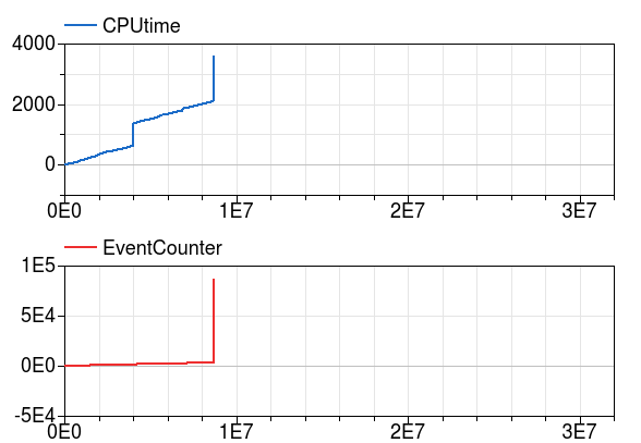
Fig. 3.6 Computing time and number of events.

As the number of events increased drastically, we enabled in Dymola in Simulation -> Setup, under the tab Debug the entry Events during simulation and simulated the model from \(t=0.9e7\) to \(t=1.0e7\) seconds. It turned out that setting the start time to \(t=0.9e7\) seconds was sufficient to reproduce the behavior; otherwise we would have had to set it to an earlier time. Inspecting Dymola’s log file dslog.txt when the simulation stalls shows that its last entries are

Expression TRet.T > amb.x_pTphi.T became true ( (TRet.T)-(amb.x_pTphi.T) = 2.9441e-08 )
Iterating to find consistent restart conditions.
      during event at Time :  9267949.854873843
Expression TRet.T > amb.x_pTphi.T became false ( (TRet.T)-(amb.x_pTphi.T) = -2.94411e-08 )
Iterating to find consistent restart conditions.
      during event at Time :  9267949.855016639
Expression TRet.T > amb.x_pTphi.T became true ( (TRet.T)-(amb.x_pTphi.T) = 2.94407e-08 )
Iterating to find consistent restart conditions.
      during event at Time :  9267949.855208419
Expression TRet.T > amb.x_pTphi.T became false ( (TRet.T)-(amb.x_pTphi.T) = -2.94406e-08 )
Iterating to find consistent restart conditions.
      during event at Time :  9267949.855351238

Hence, there is an event every few milliseconds, which explains why the simulation does not appear to be progessing. The solver does the right thing, it stops the integration, handles the event, and restarts the integration, just to encounter another event a few milliseconds later. Hence, we go back to our system model and follow the output signal of TRet.T of the return air temperature sensor, which shows that it is used in the economizer control to switch the sign of the control gain because the economizer can provide heating or cooling, depending on the ambient and return air temperature. The problematic model is shown in the figure below.

Fig. 3.7 Block diagram of part of the economizer control that computes the outside air damper control signal. This implementation triggers many events.

The events are triggered by the inequality block which changes the control, which then in turn seems to cause a slight change in the return air temperature, possibly due to numerical noise or maybe because the return fan may change its operating point as the dampers are adjusted, and hence change the heat added to the medium. Regardless, this is a bad implementation that also would cause oscillatory behavior in a real system if the sensor signal had measurement noise. Therefore, this equality comparison must be replaced by a block with hysteresis, which we did as shown in the figure below. We selected a hysteresis of \(0.2\) Kelvin, and now the model runs fine for the whole year.

Fig. 3.8 Block diagram of part of the revised economizer control that computes the outside air damper control signal.

3.4.2. State variables that dominate the error control

In a development version of the model Buildings.Examples.DualFanDualDuct.ClosedLoop (commit ef410ee), the simulation time was very slow during part of the simulation, as shown in Fig. 3.9.

Fig. 3.9 Computing time and number of events.

The number of state events did not increase in that time interval. To isolate the problem, we enabled in Dymola under Simulation -> Setup the option to log which states dominate the error (see Debug tab).

Running the simulation again gave the following output:

Integration terminated successfully at T = 1.66e+07
  Limit stepsize, Dominate error, Exceeds 10% of error  Component (#number)
               0               1            6           cooCoi.temSen_1.T (#  1)
              36               0          140           cooCoi.temSen_2.T (#  2)
              37               0            0           cooCoi.ele[1].mas.T (#  3)
              45               0            0           cooCoi.ele[2].mas.T (#  4)
              51               0            0           cooCoi.ele[3].mas.T (#  5)
              53               0            0           cooCoi.ele[4].mas.T (#  6)
           13555           13201        19064           fanSupHot.filter.x[1] (#  7)
           11905            2170        12394           fanSupHot.filter.x[2] (#  8)
             400              47          419           fanSupCol.filter.x[1] (#  9)
             420              71          521           fanSupCol.filter.x[2] (# 10)
            5082            2736         6732           fanRet.filter.x[1] (# 11)
            1979              25         4974           fanRet.filter.x[2] (# 12)
              38               0            3           TPreHeaCoi.T (# 13)
              30               0            1           TRet.T (# 14)
              38               0            3           TMix.T (# 15)
              80               0            0           TCoiCoo.T (# 16)
             305              22          275           cor.vavHot.filter.x[1] (# 18)

Hence, the state variables in the highlighted lines limit the step size significantly more often than other variables. Therefore, we removed these state variables by setting in the fan models the parameter filteredSpeed=false. After this change, the model simulates without problems.

3.5. Numerical solvers

Dymola 2021 is configured to use dassl as a default solver with a tolerance of 1E-4. We recommend to change this setting to radau with a tolerance of around 1E-6, as this generally leads to faster and more robust simulation for thermo-fluid flow systems.

Note that this is the error tolerance of the local integration time step. Most ordinary differential equation solvers only control the local integration error and not the global integration error. As a rule of thumb, the global integration error is one order of magnitude larger than the local integration error. However, the actual magnitude of the global integration error depends on the stability of the differential equation. As an extreme case, if a system is chaotic and uncontrolled, then the global integration error will grow rapidly.