2. Best Practice¶

This section explains to library users best practice in creating system models. The selected topics are based on problems that are often observed with new users of Modelica. Experienced users of Modelica may skip this section.

2.1. Organization of packages¶

When developing models, one should distinguish between a library which contains widely applicable models, such as the Buildings library, and an application-specific model which may be created for a specific building and is of limited use for other applications. It is recommended that users store application-specific models outside of the Buildings library. This will allow users to replace the Buildings library with a new version without having to change the application-specific model.

The declare the dependency of your library on Buildings version 10.0.0, use the declaration

within;
package MyLibrary

  annotation (
    uses(
      Buildings(
        version="10.0.0")
      )
   );
end MyLibrary;

If during the course of the development of application-specific models, some models turn out to be of interest for other applications, then they can be contributed to the development of the Buildings library, as described in the section Development.

2.2. Building large system models¶

When creating a large system model, it is typically easier to build the system model through the composition of subsystem models that can be tested in isolation. For example, the package Buildings.Examples.ChillerPlant.BaseClasses.Controls.Examples contains small test models that are used to test individual components in the large system model Buildings.Examples.ChillerPlant. Creating small test models typically saves time as the proper response of controls, and the proper operation of subsystems, can be tested in isolation of complex system-interactions that are often present in large models.

2.3. Propagating parameters and media packages¶

Consider a model with a pump pum and a mass flow sensor sen. Suppose that both models have a parameter m_flow_nominal for the nominal mass flow rate that needs to be set to the same value. Rather than setting these parameters individually to a numeric value, it is recommended to propagate the parameter to the top-level of the model. This allows to change the value of m_flow_nominal at one location, and then have the value be propagated to all models that reference it. The effort for the additional declaration typically pays off as changes to the model are easier and more robust.

To propagate parameters, instead of using the declaration

Pump pum(m_flow_nominal=0.1) "Pump";
TemperatureSensor sen(m_flow_nominal=0.1) "Sensor";

use

Modelica.Units.SI.MassFlowRate m_flow_nominal = 0.1 "Nominal mass flow rate";
Pump pum(m_flow_nominal=m_flow_nominal) "Pump";
TemperatureSensor sen(m_flow_nominal=m_flow_nominal) "Sensor";

Propagating parameters and packages is also recommended for medium definitions. This can be done by using the declaration

replaceable package Medium = Modelica.Media.Interfaces.PartialMedium
  "Medium model for air" annotation (choicesAllMatching=true);

Here, the optional annotation annotation (choicesAllMatching=true) is added which causes a GUI to show a drop-down menu with all medium models that extend from Modelica.Media.Interfaces.PartialMedium.

If the above sensor requires a medium model, which is likely the case, its declaration would be

TemperatureSensor sen(redeclare package Medium = Medium,
                      m_flow_nominal=m_flow_nominal) "Sensor";

At the top-level of a system-model, one would set the Medium package to an actual media, such as by using

package Medium = Buildings.Media.PerfectGases.MoistAir "Medium model";
TemperatureSensor sen(redeclare package Medium = Medium,
                      m_flow_nominal=m_flow_nominal) "Sensor";

2.4. Thermo-fluid systems¶

In this section, we describe best practices that are specific to the modeling of thermo-fluid systems.

2.4.1. Overdetermined initialization problem and inconsistent equations¶

We will now explain how state variables, such as temperature and pressure, can be initialized.

Consider a model consisting of a mass flow source Modelica.Fluid.Sources.MassFlowSource_T, a fluid volume Buildings.Fluid.MixingVolumes.MixingVolume and a fixed boundary condition Buildings.Fluid.Sources.Boundary_pT, connected in series as shown in the figure below. Note that the instance bou implements an equation that sets the medium pressure at its port, i.e., the port pressure bou.ports.p is fixed.

_images/MixingVolumeInitialization.svg — Fig. 2.1 Schematic diagram of a flow source, a fluid volume, and a pressure source.¶

The volume allows configuring balance equations for energy and mass in four different ways. Let \(p(\cdot)\) be the pressure of the volume, \(p_0\) be the parameter for the initial pressure, \(m(\cdot)\) be the mass contained in the volume, \(\dot m_i(\cdot)\) be the mass flow rate across the i-th fluid port of the volume, \(N \in \mathbb N\) be the number of fluid ports, and \(t_0\) be the initial time. Then, the equations for the mass balance of the fluid volume can be configured as shown in the table below.

Parameter	Initialization problem	Initialization problem	Equation used during time stepping
`massDynamics`	if \(\rho = \rho(p)\)	if \(\rho \not = \rho(p)\)
`DynamicsFreeInitial`	Unspecified	Unspecified	\(dm(t)/dt = \sum_{i=1}^N \dot m_i(t)\)
`FixedInitial`	\(p(t_0)=p_0\)	Unspecified	\(dm(t)/dt = \sum_{i=1}^N \dot m_i(t)\)
`SteadyStateInitial`	\(dp(t_0)/dt = 0\)	Unspecified	\(dm(t)/dt = \sum_{i=1}^N \dot m_i(t)\)
`SteadyState`	Unspecified	Unspecified	\(0 = \sum_{i=1}^N \dot m_i(t)\)

Unspecified means that no equation is declared for the initial value \(p(t_0)\). In this situation, there can be two cases:

If a system model sets the pressure in the above model vol.p=vol.ports.p=bou.ports.p due to the connection between them, then \(p(t_0)\) of the volume is equal to bou.ports.p.
If a system model does not set the pressure (i.e., if vol and bou are not connected to each other), then the pressure starts at the value p(start=Medium.p_default), where Medium is the name of the instance of the medium model.

Since the model Buildings.Fluid.Sources.Boundary_pT fixes the pressure at its port, the initial conditions \(p(t_0)=p_0\) and \(dp(t_0)/dt = 0\) lead to an overspecified system for the model shown above. To avoid such situation, use different initial conditions, or add a flow resistance between the mixing volume and the pressure source. The flow resistance introduces an equation that relates the pressure of the mixing volume and the pressure source as a function of the mass flow rate, thereby removing the inconsistency.

Warning

The setting FixedInitial should be used with caution: Since the pressure dynamics is fast, this setting can lead to very fast transients when the simulation starts. Such transients can cause numerical problems for differential equation solvers.

Similarly, for the energy balance, let \(U(\cdot)\) be the energy stored in the volume, \(T(\cdot)\) be the temperature of the volume, \(m_i(\cdot)\) be the mass flow rate that carries the specific enthalpy per unit mass \(h_i(\cdot)\) across the i-th fluid connector of the volume, and let \(Q(\cdot)\) be the heat flow at the heat port of the volume. Then, the energy balance can be configured as shown in the table below.

Parameter `energyDynamics`	Initialization problem	Equation used during time stepping
`DynamicsFreeInitial`	Unspecified	\(dU(t)/dt = \sum_{i=1}^N \dot m_i(t) \, h_i(t) + \dot Q(t)\)
`FixedInitial`	\(T(t_0)=T_0\)	\(dU(t)/dt = \sum_{i=1}^N \dot m_i(t) \, h_i(t) + \dot Q(t)\)
`SteadyStateInitial`	\(dT(t_0)/dt = 0\)	\(dU(t)/dt = \sum_{i=1}^N \dot m_i(t) \, h_i(t) + \dot Q(t)\)
`SteadyState`	Unspecified	\(0 = \sum_{i=1}^N \dot m_i(t) \, h_i(t) + \dot Q(t)\)

Unspecified means that no equation is declared for \(T(t_0)\). In this situation, there can be two cases:

If a system model sets the temperature (i.e. if in the model the heat port of vol is connected to a fixed temperature), then \(T(t_0)\) of the volume would be equal to the temperature connected to this port.
If a system model does not set the temperature, then the temperature starts at the value T(start=Medium.T_default), where Medium is the medium model.

Note

Selecting SteadyState for the energy balance and not SteadyState for the mass balance can lead to inconsistent equations. The model will check for this situation and stop the translation with an error message. To see why the equations are inconsistent, consider a volume with two fluid ports and no heat port. Then, it is possible that \(\dot m_1(t) \not = 0\) and \(\dot m_2(t) = 0\), since \(dm(t)/dt = \dot m_1(t) + \dot m_2(t)\). However, the energy balance equation is \(0 = \sum_{i=1}^2 \dot m_i(t) \, h_i(t) + \dot Q(t)\), with \(\dot Q(t) = 0\) because there is no heat port. Therefore, we obtain \(0 = \dot m_1(t) \, h_1(t)\), which is inconsistent.
Unlike the case with the pressure initialization, the temperature in the model bou does not lead to vol.T = bou.T at initial time, because physics allows the temperatures in bou and vol to be different.

The equations for the mass fraction dynamics (such as the water vapor concentration), and the trace substance dynamics (such as carbon dioxide concentration), are similar to the energy equations.

Let \(X(\cdot)\) be the mass of the species in the volume, \(m(t_0)\) be the initial mass of the volume, \(x_0\) be the user-selected species concentration in the volume, \(x_i(\cdot)\) be the species concentration at the i-th fluid port, and \(\dot X(\cdot)\) be the species added from the outside, for example the water vapor added by a humidifier. Then, the substance dynamics can be configured as shown in the table below.

Parameter `massDynamics`	Initialization problem	Equation used during time stepping
`DynamicsFreeInitial`	Unspecified	\(dX(t)/dt = \sum_{i=1}^N \dot m_i(t) \, x_i(t) + \dot X(t)\)
`FixedInitial`	\(X(t_0)= m(t_0) \, x_0\)	\(dX(t)/dt = \sum_{i=1}^N \dot m_i(t) \, x_i(t) + \dot X(t)\)
`SteadyStateInitial`	\(dX(t_0)/dt = 0\)	\(dX(t)/dt = \sum_{i=1}^N \dot m_i(t) \, x_i(t) + \dot X(t)\)
`SteadyState`	Unspecified	\(0 = \sum_{i=1}^N \dot m_i(t) \, x_i(t) + \dot X(t)\)

The equations for the trace substance dynamics are identical to the equations for the substance dynamics, if \(X(\cdot), \, \dot X(\cdot)\) and \(x_i(\cdot)\) are replaced with \(C(\cdot), \, \dot C(\cdot)\) and \(c_i(\cdot)\), where \(C(\cdot)\) is the mass of the trace substances in the volume, \(c_i(\cdot)\) is the trace substance concentration at the i-th fluid port and \(\dot C(\cdot)\) is the trace substance mass flow rate added from the outside. Therefore, energy, mass fraction and trace substances have identical equations and configurations.

2.4.2. Modeling of fluid junctions¶

In Modelica, connecting fluid ports as shown below leads to ideal mixing at the junction. In some situation, such as the configuration below, connecting multiple connectors to a fluid port represents the physical phenomena that was intended to model.

_images/fluidJunctionMixing.svg — Fig. 2.2 Connection of three components without explicitly introducing a flow junction model.¶

However, in more complex flow configurations, one may want to explicitly control what branches of a piping or duct network mix. This may be achieved by using an instance of the model Junction as shown in the left figure below, which is derived from the test model BoilerPolynomialClosedLoop

_images/fluidJunctionMixingSplitter.svg — Fig. 2.3 Correct (a) and wrong (b) and (c) connection of components with use of a flow junction model.¶

In Fig. 2.3 (a), the mixing points have been correctly defined by use of the model Junction. However, in Fig. 2.3 (b), all connections are made to the port of the instance spl2. This results in the same configuration as is shown in Fig. 2.3 (c). This is certainly not the intention of the modeler, as this causes all flows to be mixed in the port. Consequently, the valve will received fluid at this mixing temperature rather than at the return temperature from the radiator, e.g., the system model is wrong.

The overhead for the simulation of these flow junctions can be reduced by setting the nominal pressure drop of flow junction model to zero, which will remove the pressure drop equation.

2.4.3. Use of sensors in fluid flow systems¶

When selecting a sensor model, a distinction needs to be made whether the measured quantity depends on the direction of the flow or not. If the quantity depends on the flow direction, such as temperature or relative humidity, then sensors with two ports from the Buildings.Fluid.Sensors library should be used. These sensors have a more efficient implementation than sensors with one port for situations where the flow reverses its direction. The proper use sensors is described in the User’s Guide of the Buildings.Fluid.Sensors package.

2.4.4. Reference pressure for incompressible fluids such as water¶

This section explains how to set a reference pressure for fluids that model the flow as incompressible flow, such as Buildings.Media.Water and Buildings.Media.Antifreeze.PropyleneGlycolWater.

Consider the flow circuit shown in Fig. 2.4 that consists of a pump or fan, a flow resistance and a volume.

_images/flowCircuit.svg — Fig. 2.4 Schematic diagram of a flow circuit without means to set a reference pressure, or to account for thermal expansion of the fluid.¶

When this model is used with a medium model that models compressible flow, then the model is well defined because the gas medium implements an equation that relates density to pressure.

However, when the medium model is changed to a model that models incompressible flow, then there is no equation that can be used to compute the pressure. In this situation, attempting to translate the model leads, in Dymola, to the following error message:

The DAE has 151 scalar unknowns and 151 scalar equations.
Error: The model FlowCircuit is structurally singular.
The problem is structurally singular for the element type Real.
The number of scalar Real unknown elements are 58.
The number of scalar Real equation elements are 58.

Similarly, if the medium model Buildings.Media.Specialized.Water.TemperatureDependentDensity, which models density as a function of pressure and enthalpy, is used, then the model is well-defined, but the pressure increases the longer the pump runs. The reason is that the pump adds heat to the water. When the water temperature increases from \(20^\circ \mathrm C\) to \(40^\circ \mathrm C\), the pressure increases from \(1 \, \mathrm{bars}\) to \(150 \, \mathrm{bars}\).

To avoid this singularity or increase in pressure, use a model that imposes a pressure source and that accounts for the expansion of the fluid. For example, use Buildings.Fluid.Sources.Boundary_pT to form the system model shown in Fig. 2.5.

_images/flowCircuitWithBoundary.svg — Fig. 2.5 Schematic diagram of a flow circuit with a model that provides a reference presssure.¶

Alternatively, you may use Buildings.Fluid.Storage.ExpansionVessel, but Buildings.Fluid.Sources.Boundary_pT usually leads to simpler equations than Buildings.Fluid.Storage.ExpansionVessel. Note that the medium that flows out of the fluid port of Buildings.Fluid.Sources.Boundary_pT is at a fixed temperature, while the model Buildings.Fluid.Storage.ExpansionVessel conserves energy. However, since the thermal expansion of the fluid is usually small, this effect can be neglected in most building HVAC applications.

Note

In each water circuit, there must be exactly on instance of Buildings.Fluid.Sources.Boundary_pT, or instance of Buildings.Fluid.Storage.ExpansionVessel.

If there is more than one such device, then there are multiple points in the system that set the reference static pressure. This will affect the distribution of the mass flow rate.

Note

If Dymola fails to translate a model with the error message:

Error: The initialization problem is overspecified for variables
of element type Real
The initial equation
...
refers to variables, which are all knowns.
To correct it you can remove this equation.

then the initialization problem is overspecified. To avoid this, set

energyDynamics = Modelica.Fluid.Types.Dynamics.DynamicsFreeInitial;
massDynamics = Modelica.Fluid.Types.Dynamics.DynamicsFreeInitial;

in the instances of the components that contain fluid volumes.

2.4.5. Nominal Values¶

Most components have a parameters for the nominal operating conditions. These parameters have names that end in _nominal and they should be set to the values that the component typically has if it is operated at full load or design conditions. Depending on the model, these parameters are used differently, and the respective model documentation or code should be consulted for details. However, the table below shows typical use of parameters in various model to help the user understand how they are used.

Parameter	Model	Functionality
`m_flow_nominal` `dp_nominal`	Flow resistance models.	These parameters may be used to define a point on the flow rate versus pressure drop curve. For other mass flow rates, the pressure drop is typically adjusted using similarity laws. See PressureDrop.
`m_flow_nominal` `m_flow_small`	Sensors. Volumes. Heat exchangers.	Some of these models set `m_flow_small=1E-4*abs(m_flow_nominal)` as the default value. Then, m_flow_small is used to regularize, or replace, equations when the mass flow rate is smaller than `m_flow_small` in magnitude. This is needed to improve the numerical properties of the model. The error in the results is negligible for typical applications, because at flow rates below 0.01% from the design flow rate, most model assumptions are not applicable anyways, and the HVAC system is not operated in this region. Modelica simulates in the continuous-time domain, thus such small flow rates can occur, and therefore models are implemented in such a way that they are numerically well-behaved for zero or near-zero flow rates.
`tau` `m_flow_nominal`	Sensors. Volumes. Heat exchangers. Chillers.	Because Modelica simulates in the continuous-time domain, dynamic models are in general numerically more efficient than steady-state models. However, dynamic models require product data that are generally not published by manufacturers. Examples include the volume of fluid that is contained in a device, and the weight of heat exchangers. In addition, other effects such as transport delays in pipes and heat exchangers of a chiller are generally unknown and require detailed geometry that is typically not available during the design stage. To circumvent this problem, many models take as a parameter the time constant `tau` and lump all its thermal mass into a fluid volume. The time constant `tau` can be understood as the time constant that one would observe if the input to the component has a step change, and the mass flow rate of the component is equal to `m_flow_nominal`. Using these two values and the fluid density `rho`, components adjust their fluid volume `V=m_flow_nominal tau/rho` because having such a volume gives the specified time response. For most components, engineering experience can be used to estimate a reasonable value for `tau`, and where generally applicable values can be used, components already set a default value for `tau.` See for example WetCoilDiscretized.

Parameter

Model

Functionality

m_flow_nominal dp_nominal

Flow resistance models.

These parameters may be used to define a point on the flow rate versus pressure drop curve. For other mass flow rates, the pressure drop is typically adjusted using similarity laws. See PressureDrop.

m_flow_nominal m_flow_small

Sensors.
Volumes.
Heat exchangers.

Some of these models set m_flow_small=1E-4*abs(m_flow_nominal) as the default value. Then, m_flow_small is used to regularize, or replace, equations when the mass flow rate is smaller than m_flow_small in magnitude. This is needed to improve the numerical properties of the model. The error in the results is negligible for typical applications, because at flow rates below 0.01% from the design flow rate, most model assumptions are not applicable anyways, and the HVAC system is not operated in this region. Modelica simulates in the continuous-time domain, thus such small flow rates can occur, and therefore models are implemented in such a way that they are numerically well-behaved for zero or near-zero flow rates.

tau m_flow_nominal

Sensors.
Volumes.
Heat exchangers.
Chillers.

Because Modelica simulates in the continuous-time domain, dynamic models are in general numerically more efficient than steady-state models. However, dynamic models require product data that are generally not published by manufacturers. Examples include the volume of fluid that is contained in a device, and the weight of heat exchangers. In addition, other effects such as transport delays in pipes and heat exchangers of a chiller are generally unknown and require detailed geometry that is typically not available during the design stage.

To circumvent this problem, many models take as a parameter the time constant tau and lump all its thermal mass into a fluid volume. The time constant tau can be understood as the time constant that one would observe if the input to the component has a step change, and the mass flow rate of the component is equal to m_flow_nominal. Using these two values and the fluid density rho, components adjust their fluid volume V=m_flow_nominal tau/rho because having such a volume gives the specified time response. For most components, engineering experience can be used to estimate a reasonable value for tau, and where generally applicable values can be used, components already set a default value for tau. See for example WetCoilDiscretized.

2.5. Controls¶

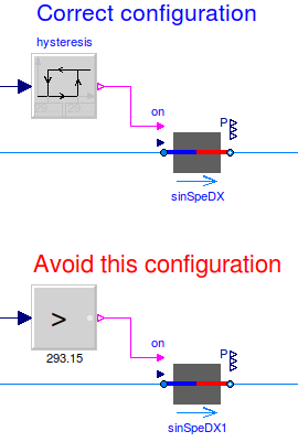
_images/controlHysteresis.png — Fig. 2.6 Schematic diagram of a controller that switches a coil on and off. In the top configuration, the hysteresis avoids numerical problems (and short-cycling) if the control input remains close to the set point. The bottom configuration uses an inequality comparison Modelica.Blocks.Logical.GreaterThreshold which has no hysteresis. This can cause the integration to stall if the input signal to the threshold block is the solution of an iterative solver and remains around 293.15 Kelvin.¶

When implementing an on/off controller, always use a controller with hysteresis such as shown in the top configuration of the model above. If no hysteresis is used, then numerical problems can occur if the variable that is input to the controller depends on a variable that is computed by an iterative algorithm. To avoid this, the Modelica Buildings Library contains inequality blocks such as Buildings.Controls.OBC.CDL.Reals.GreaterThreshold that have a hysteresis parameter.

Examples of a iterative algorithms are nonlinear equation solvers or time integration algorithms with variable step size (such as the radau and dassl solver in Dymola). The problem is caused as follows: Let \(T(t) \in \Re\) be the input into a controller, such as a room air temperature. If \(T(t)\) is the state variable computed by solving a differential equation, or if \(T(t)\) depends on a variable that needs to be solved for iteratively, then \(T(t)\) can only be approximated by some approximation \(T^*(\epsilon, t)\), where \(\epsilon\) is the solver tolerance. Even if the system is at an equilibrium, the solver can cause the value of \(T^*(\epsilon, t)\) to slightly change from one iteration to another. Hence, \(T^*(\epsilon, t)\) can exhibit what is called numerical noise. Now, if \(T^*(\epsilon, t)\) is used to switch a heater on and off whenever it crosses at set point temperature, and if \(T(t)\) happens to be at an equilibrium near the set point temperature, then the heater can switch on and off rapidly due to the numerical noise. This can cause the time integration to stall.

To illustrate this problem, try to simulate

model Unstable
  Real x(start=0.1);
equation
  der(x) = if x > 0 then -1 else 1;
end Unstable;

In Dymola 2013, as expected the model stalls at \(t=0.1\) because the if-then-else construct triggers an event iteration whenever \(x\) crosses zero.

Warning

Never use an inequality comparison without a hysteresis or a time delay if the variable that is used in the inequality test

is computed using an iterative solver, or
is obtained from a measurement and hence can contain measurement noise.

An exception is a sampled value because the output of a sampler remains constant until the next sampling instant.

See Examples for how to debug and correct slow simulations for what can happen in such tests.

2.6. Start values of iteration variables¶

When computing numerical solutions to systems of nonlinear equations, a Newton-based solver is typically used. Such solvers have a higher success of convergence if good start values are provided for the iteration variables. In Dymola, to see what start values are used, one can enter on the simulation tab the command

Advanced.LogStartValuesForIterationVariables = true;

Then, when a model is translated, for example using

translateModel("Buildings.Fluid.Boilers.Examples.BoilerPolynomialClosedLoop");

an output of the form

Start values for iteration variables:
 val.res1.dp(start = 3000.0)
 val.res3.dp(start = 3000.0)

is produced. This shows the iteration variables and their start values. These start values can be overwritten in the model.