Modelica.Fluid.Utilities

Information

Extends from Modelica.Icons.Package (Icon for standard packages).

Package Content

Name	Description
checkBoundary	Check whether boundary definition is correct
regRoot	Anti-symmetric square root approximation with finite derivative in the origin
regRoot_der	Derivative of regRoot
regSquare	Anti-symmetric square approximation with non-zero derivative in the origin
regPow	Anti-symmetric power approximation with non-zero derivative in the origin
regRoot2	Anti-symmetric approximation of square root with discontinuous factor so that the first derivative is finite and continuous
regSquare2	Anti-symmetric approximation of square with discontinuous factor so that the first derivative is non-zero and is continuous
regStep	Approximation of a general step, such that the characteristic is continuous and differentiable
evaluatePoly3_derivativeAtZero	Evaluate polynomial of order 3 that passes the origin with a predefined derivative
regFun3	Co-monotonic and C1 smooth regularization function
cubicHermite	Evaluate a cubic Hermite spline
cubicHermite_withDerivative	Evaluate a cubic Hermite spline, return value and derivative

Modelica.Fluid.Utilities.checkBoundary

Information

Inputs

Type	Name	Default	Description
String	mediumName
String	substanceNames[:]		Names of substances
Boolean	singleState
Boolean	define_p
Real	X_boundary[:]
String	modelName	"??? boundary ???"

Modelica definition

function checkBoundary "Check whether boundary definition is correct"
  extends Modelica.Icons.Function;
  input String mediumName;
  input String substanceNames[:] "Names of substances";
  input Boolean singleState;
  input Boolean define_p;
  input Real X_boundary[:];
  input String modelName = "??? boundary ???";
protected 
  Integer nX = size(X_boundary,1);
  String X_str;
algorithm 
  assert(not singleState or singleState and define_p, "
Wrong value of parameter define_p (= false) in model \"" + modelName + "\":
The selected medium \""
                      + mediumName + "\" has Medium.singleState=true.
Therefore, an boundary density cannot be defined and
define_p = true is required.
");

  for i in 1:nX loop
    assert(X_boundary[i] >= 0.0, "
Wrong boundary mass fractions in medium \""
+ mediumName + "\" in model \"" + modelName + "\":
The boundary value X_boundary("
                            + String(i) + ") = " + String(
      X_boundary[i]) + "
is negative. It must be positive.
");
  end for;

  if nX > 0 and abs(sum(X_boundary) - 1.0) > 1.e-10 then
     X_str :="";
     for i in 1:nX loop
        X_str :=X_str + "   X_boundary[" + String(i) + "] = " + String(X_boundary[
        i]) + " \"" + substanceNames[i] + "\"\n";
     end for;
     Modelica.Utilities.Streams.error(
        "The boundary mass fractions in medium \"" + mediumName + "\" in model \"" + modelName + "\"\n" +
        "do not sum up to 1. Instead, sum(X_boundary) = " + String(sum(X_boundary)) + ":\n"
        + X_str);
  end if;
end checkBoundary;

Modelica.Fluid.Utilities.regRoot

Information

Function	Approximation	Range
y = regRoot(x)	y ~= sqrt(abs(x))*sgn(x)	abs(x) >>delta
y = regRoot(x)	y ~= x/sqrt(delta)	abs(x) << delta

With the default value of delta=0.01, the difference between sqrt(x) and regRoot(x) is 16% around x=0.01, 0.25% around x=0.1 and 0.0025% around x=1.

Extends from Modelica.Icons.Function (Icon for functions).

Inputs

Type	Name	Default	Description
Real	x
Real	delta	0.01	Range of significant deviation from sqrt(abs(x))*sgn(x)

Outputs

Type	Name	Description
Real	y

Modelica definition

function regRoot 
  "Anti-symmetric square root approximation with finite derivative in the origin"
  annotation(derivative=Utilities.regRoot_der);
  extends Modelica.Icons.Function;
  input Real x;
  input Real delta=0.01 
    "Range of significant deviation from sqrt(abs(x))*sgn(x)";
  output Real y;
algorithm 
  y := x/(x*x+delta*delta)^0.25;

end regRoot;

Modelica.Fluid.Utilities.regRoot_der

Information

Extends from Modelica.Icons.Function (Icon for functions).

Inputs

Type	Name	Default	Description
Real	x
Real	delta	0.01	Range of significant deviation from sqrt(x)
Real	dx		Derivative of x

Outputs

Type	Name	Description
Real	dy

Modelica definition

function regRoot_der "Derivative of regRoot"
  extends Modelica.Icons.Function;
  input Real x;
  input Real delta=0.01 "Range of significant deviation from sqrt(x)";
  input Real dx "Derivative of x";
  output Real dy;
algorithm 
  dy := dx*0.5*(x*x+2*delta*delta)/((x*x+delta*delta)^1.25);

end regRoot_der;

Modelica.Fluid.Utilities.regSquare

Information

Function	Approximation	Range
y = regSquare(x)	y ~= x^2*sgn(x)	abs(x) >>delta
y = regSquare(x)	y ~= x*delta	abs(x) << delta

With the default value of delta=0.01, the difference between x^2 and regSquare(x) is 41% around x=0.01, 0.4% around x=0.1 and 0.005% around x=1.

Extends from Modelica.Icons.Function (Icon for functions).

Inputs

Type	Name	Default	Description
Real	x
Real	delta	0.01	Range of significant deviation from x^2*sgn(x)

Outputs

Type	Name	Description
Real	y

Modelica definition

function regSquare 
  "Anti-symmetric square approximation with non-zero derivative in the origin"
  extends Modelica.Icons.Function;
  input Real x;
  input Real delta=0.01 "Range of significant deviation from x^2*sgn(x)";
  output Real y;
algorithm 
  y := x*sqrt(x*x+delta*delta);

end regSquare;

Modelica.Fluid.Utilities.regPow

Information

Function	Approximation	Range
y = regPow(x)	y ~= abs(x)^a*sgn(x)	abs(x) >>delta
y = regPow(x)	y ~= x*delta^(a-1)	abs(x) << delta

Extends from Modelica.Icons.Function (Icon for functions).

Inputs

Type	Name	Default	Description
Real	x
Real	a
Real	delta	0.01	Range of significant deviation from x^a*sgn(x)

Outputs

Type	Name	Description
Real	y

Modelica definition

function regPow 
  "Anti-symmetric power approximation with non-zero derivative in the origin"
  extends Modelica.Icons.Function;
  input Real x;
  input Real a;
  input Real delta=0.01 "Range of significant deviation from x^a*sgn(x)";
  output Real y;
algorithm 
  y := x*(x*x+delta*delta)^((a-1)/2);

end regPow;

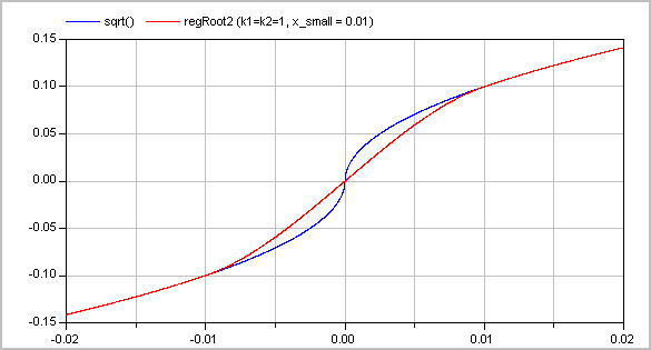
Modelica.Fluid.Utilities.regRoot2

Information

Approximates the function

   y = if x ≥ 0 then sqrt(k1*x) else -sqrt(k2*abs(x)), with k1, k2 ≥ 0

in such a way that within the region -x_small ≤ x ≤ x_small, the function is described by two polynomials of third order (one in the region -x_small .. 0 and one within the region 0 .. x_small) such that

• The derivative at x=0 is finite.
• The overall function is continuous with a continuous first derivative everywhere.
• If parameter use_yd0 = false, the two polynomials are constructed such that the second derivatives at x=0 are identical. If use_yd0 = true, the derivative at x=0 is explicitly provided via the additional argument yd0. If necessary, the derivative yd0 is automatically reduced in order that the polynomials are strict monotonically increasing [Fritsch and Carlson, 1980].

Typical screenshots for two different configurations are shown below. The first one with k1=k2=1:

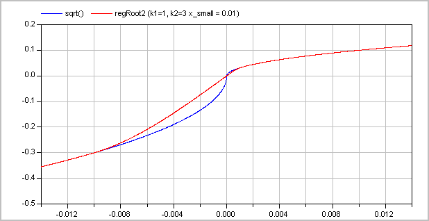
and the second one with k1=1 and k2=3:

The (smooth) derivative of the function with k1=1, k2=3 is shown in the next figure:

Literature

Fritsch F.N. and Carlson R.E. (1980):

Monotone piecewise cubic interpolation. SIAM J. Numerc. Anal., Vol. 17, No. 2, April 1980, pp. 238-246

Extends from Modelica.Icons.Function (Icon for functions).

Inputs

Type	Name	Default	Description
Real	x		abscissa value
Real	x_small	0.01	approximation of function for |x| <= x_small
Real	k1	1	y = if x>=0 then sqrt(k1*x) else -sqrt(k2*|x|)
Real	k2	1	y = if x>=0 then sqrt(k1*x) else -sqrt(k2*|x|)
Boolean	use_yd0	false	= true, if yd0 shall be used
Real	yd0	1	Desired derivative at x=0: dy/dx = yd0

Outputs

Type	Name	Description
Real	y	ordinate value

Modelica definition

function regRoot2 
  "Anti-symmetric approximation of square root with discontinuous factor so that the first derivative is finite and continuous"

  extends Modelica.Icons.Function;
  input Real x "abscissa value";
  input Real x_small(min=0)=0.01 "approximation of function for |x| <= x_small";
  input Real k1(min=0)=1 "y = if x>=0 then sqrt(k1*x) else -sqrt(k2*|x|)";
  input Real k2(min=0)=1 "y = if x>=0 then sqrt(k1*x) else -sqrt(k2*|x|)";
  input Boolean use_yd0 = false "= true, if yd0 shall be used";
  input Real yd0(min=0)=1 "Desired derivative at x=0: dy/dx = yd0";
  output Real y "ordinate value";
protected 
  encapsulated function regRoot2_utility 
    "Interpolating with two 3-order polynomials with a prescribed derivative at x=0"
    import Modelica.Fluid.Utilities.evaluatePoly3_derivativeAtZero;
     input Real x;
     input Real x1 "approximation of function abs(x) < x1";
     input Real k1 "y = if x>=0 then sqrt(k1*x) else -sqrt(k2*|x|); k1 >= k2";
     input Real k2 "y = if x>=0 then sqrt(k1*x) else -sqrt(k2*|x|))";
     input Boolean use_yd0 "= true, if yd0 shall be used";
     input Real yd0(min=0) "Desired derivative at x=0: dy/dx = yd0";
     output Real y;
  protected 
     Real x2;
     Real xsqrt1;
     Real xsqrt2;
     Real y1;
     Real y2;
     Real y1d;
     Real y2d;
     Real w;
     Real y0d;
     Real w1;
     Real w2;
  algorithm 
     if k2 > 0 then
        x2 :=-x1*(k2/k1);
     else
        x2 := -x1;
     end if;

     if x <= x2 then
        y := -sqrt(k2*abs(x));
     else
        y1 :=sqrt(k1*x1);
        y2 :=-sqrt(k2*abs(x2));
        y1d :=sqrt(k1/x1)/2;
        y2d :=sqrt(k2/abs(x2))/2;

        if use_yd0 then
           y0d :=yd0;
        else
           /* Determine derivative, such that first and second derivative
              of left and right polynomial are identical at x=0:
           _
           Basic equations:
              y_right = a1*(x/x1) + a2*(x/x1)^2 + a3*(x/x1)^3
              y_left  = b1*(x/x2) + b2*(x/x2)^2 + b3*(x/x2)^3
              yd_right*x1 = a1 + 2*a2*(x/x1) + 3*a3*(x/x1)^2
              yd_left *x2 = b1 + 2*b2*(x/x2) + 3*b3*(x/x2)^2
              ydd_right*x1^2 = 2*a2 + 6*a3*(x/x1)
              ydd_left *x2^2 = 2*b2 + 6*b3*(x/x2)
           _
           Conditions (6 equations for 6 unknowns):
                     y1 = a1 + a2 + a3
                     y2 = b1 + b2 + b3
                 y1d*x1 = a1 + 2*a2 + 3*a3
                 y2d*x2 = b1 + 2*b2 + 3*b3
                    y0d = a1/x1 = b1/x2
                   y0dd = 2*a2/x1^2 = 2*b2/x2^2
           _
           Derived equations:
              b1 = a1*x2/x1
              b2 = a2*(x2/x1)^2
              b3 = y2 - b1 - b2
                 = y2 - a1*(x2/x1) - a2*(x2/x1)^2
              a3 = y1 - a1 - a2
           _
           Remaining equations
              y1d*x1 = a1 + 2*a2 + 3*(y1 - a1 - a2)
                     = 3*y1 - 2*a1 - a2
              y2d*x2 = a1*(x2/x1) + 2*a2*(x2/x1)^2 +
                       3*(y2 - a1*(x2/x1) - a2*(x2/x1)^2)
                     = 3*y2 - 2*a1*(x2/x1) - a2*(x2/x1)^2
              y0d    = a1/x1
           _
           Solving these equations results in y0d below
           (note, the denominator "(1-w)" is always non-zero, because w is negative)
           */
           w :=x2/x1;
           y0d := ( (3*y2 - x2*y2d)/w - (3*y1 - x1*y1d)*w) /(2*x1*(1 - w));
        end if;

        /* Modify derivative y0d, such that the polynomial is
           monotonically increasing. A sufficient condition is
             0 <= y0d <= sqrt(8.75*k_i/|x_i|)
        */
        w1 :=sqrt(8.75*k1/x1);
        w2 :=sqrt(8.75*k2/abs(x2));
        y0d :=min(y0d, 0.9*min(w1, w2));

        /* Perform interpolation in scaled polynomial:
           y_new = y/y1
           x_new = x/x1
        */
        y := y1*(if x >= 0 then evaluatePoly3_derivativeAtZero(x/x1,1,1,y1d*x1/y1,y0d*x1/y1) else 
                                evaluatePoly3_derivativeAtZero(x/x1,x2/x1,y2/y1,y2d*x1/y1,y0d*x1/y1));
     end if;
  end regRoot2_utility;
algorithm 
  y := smooth(2, if x >= x_small then sqrt(k1*x) else 
                 if x <= -x_small then -sqrt(k2*abs(x)) else 
                 if k1 >= k2 then regRoot2_utility(x,x_small,k1,k2,use_yd0,yd0) else 
                                 -regRoot2_utility(-x,x_small,k2,k1,use_yd0,yd0));
end regRoot2;

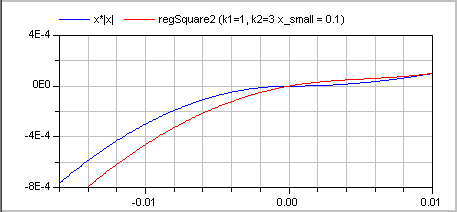
Modelica.Fluid.Utilities.regSquare2

Information

Approximates the function

   y = if x ≥ 0 then k1*x*x else -k2*x*x, with k1, k2 > 0

in such a way that within the region -x_small ≤ x ≤ x_small, the function is described by two polynomials of third order (one in the region -x_small .. 0 and one within the region 0 .. x_small) such that

• The derivative at x=0 is non-zero (in order that the inverse of the function does not have an infinite derivative).
• The overall function is continuous with a continuous first derivative everywhere.
• If parameter use_yd0 = false, the two polynomials are constructed such that the second derivatives at x=0 are identical. If use_yd0 = true, the derivative at x=0 is explicitly provided via the additional argument yd0. If necessary, the derivative yd0 is automatically reduced in order that the polynomials are strict monotonically increasing [Fritsch and Carlson, 1980].

A typical screenshot for k1=1, k2=3 is shown in the next figure:

The (smooth, non-zero) derivative of the function with k1=1, k2=3 is shown in the next figure:

Literature

Fritsch F.N. and Carlson R.E. (1980):

Monotone piecewise cubic interpolation. SIAM J. Numerc. Anal., Vol. 17, No. 2, April 1980, pp. 238-246

Extends from Modelica.Icons.Function (Icon for functions).

Inputs

Type	Name	Default	Description
Real	x		abscissa value
Real	x_small	0.01	approximation of function for |x| <= x_small
Real	k1	1	y = (if x>=0 then k1 else k2)*x*|x|
Real	k2	1	y = (if x>=0 then k1 else k2)*x*|x|
Boolean	use_yd0	false	= true, if yd0 shall be used
Real	yd0	1	Desired derivative at x=0: dy/dx = yd0

Outputs

Type	Name	Description
Real	y	ordinate value

Modelica definition

function regSquare2 
  "Anti-symmetric approximation of square with discontinuous factor so that the first derivative is non-zero and is continuous"
  extends Modelica.Icons.Function;
  input Real x "abscissa value";
  input Real x_small(min=0)=0.01 "approximation of function for |x| <= x_small";
  input Real k1(min=0)=1 "y = (if x>=0 then k1 else k2)*x*|x|";
  input Real k2(min=0)=1 "y = (if x>=0 then k1 else k2)*x*|x|";
  input Boolean use_yd0 = false "= true, if yd0 shall be used";
  input Real yd0(min=0)=1 "Desired derivative at x=0: dy/dx = yd0";
  output Real y "ordinate value";
protected 
  encapsulated function regSquare2_utility 
    "Interpolating with two 3-order polynomials with a prescribed derivative at x=0"
    import Modelica.Fluid.Utilities.evaluatePoly3_derivativeAtZero;
     input Real x;
     input Real x1 "approximation of function abs(x) < x1";
     input Real k1 "y = (if x>=0 then k1 else -k2)*x*|x|; k1 >= k2";
     input Real k2 "y = (if x>=0 then k1 else -k2)*x*|x|";
     input Boolean use_yd0 = false "= true, if yd0 shall be used";
     input Real yd0(min=0)=1 "Desired derivative at x=0: dy/dx = yd0";
     output Real y;
  protected 
     Real x2;
     Real y1;
     Real y2;
     Real y1d;
     Real y2d;
     Real w;
     Real w1;
     Real w2;
     Real y0d;
     Real ww;
  algorithm 
     // x2 :=-x1*(k2/k1)^2;
     x2 := -x1;
     if x <= x2 then
        y := -k2*x^2;
     else
         y1 := k1*x1^2;
         y2 :=-k2*x2^2;
        y1d := k1*2*x1;
        y2d :=-k2*2*x2;
        if use_yd0 then
           y0d :=yd0;
        else
           /* Determine derivative, such that first and second derivative
              of left and right polynomial are identical at x=0:
              see derivation in function regRoot2
           */
           w :=x2/x1;
           y0d := ( (3*y2 - x2*y2d)/w - (3*y1 - x1*y1d)*w) /(2*x1*(1 - w));
        end if;

        /* Modify derivative y0d, such that the polynomial is
           monotonically increasing. A sufficient condition is
             0 <= y0d <= sqrt(5)*k_i*|x_i|
        */
        w1 :=sqrt(5)*k1*x1;
        w2 :=sqrt(5)*k2*abs(x2);
        // y0d :=min(y0d, 0.9*min(w1, w2));
        ww :=0.9*(if w1 < w2 then w1 else w2);
        if ww < y0d then
           y0d :=ww;
        end if;
        y := if x >= 0 then evaluatePoly3_derivativeAtZero(x,x1,y1,y1d,y0d) else 
                            evaluatePoly3_derivativeAtZero(x,x2,y2,y2d,y0d);
     end if;
  end regSquare2_utility;
algorithm 
  y := smooth(2,if x >= x_small then k1*x^2 else 
                if x <= -x_small then -k2*x^2 else 
                if k1 >= k2 then regSquare2_utility(x,x_small,k1,k2,use_yd0,yd0) else 
                                -regSquare2_utility(-x,x_small,k2,k1,use_yd0,yd0));
end regSquare2;

Modelica.Fluid.Utilities.regStep

Information

This function is used to approximate the equation

    y = if x > 0 then y1 else y2;

by a smooth characteristic, so that the expression is continuous and differentiable:

   y = smooth(1, if x >  x_small then y1 else
                 if x < -x_small then y2 else f(y1, y2));

In the region -x_small < x < x_small a 2nd order polynomial is used for a smooth transition from y1 to y2.

Extends from Modelica.Icons.Function (Icon for functions).

Inputs

Type	Name	Default	Description
Real	x		Abscissa value
Real	y1		Ordinate value for x > 0
Real	y2		Ordinate value for x < 0
Real	x_small	1e-5	Approximation of step for -x_small <= x <= x_small; x_small >= 0 required

Outputs

Type	Name	Description
Real	y	Ordinate value to approximate y = if x > 0 then y1 else y2

Modelica definition

function regStep 
  "Approximation of a general step, such that the characteristic is continuous and differentiable"
  extends Modelica.Icons.Function;
  input Real x "Abscissa value";
  input Real y1 "Ordinate value for x > 0";
  input Real y2 "Ordinate value for x < 0";
  input Real x_small(min=0) = 1e-5 
    "Approximation of step for -x_small <= x <= x_small; x_small >= 0 required";
  output Real y "Ordinate value to approximate y = if x > 0 then y1 else y2";
algorithm 
  y := smooth(1, if x >  x_small then y1 else 
                 if x < -x_small then y2 else 
                 if x_small > 0 then (x/x_small)*((x/x_small)^2 - 3)*(y2-y1)/4 + (y1+y2)/2 else (y1+y2)/2);
end regStep;

Modelica.Fluid.Utilities.evaluatePoly3_derivativeAtZero

Information

Extends from Modelica.Icons.Function (Icon for functions).

Inputs

Type	Name	Default	Description
Real	x		Value for which polynomial shall be evaluated
Real	x1		Abscissa value
Real	y1		y1=f(x1)
Real	y1d		First derivative at y1
Real	y0d		First derivative at f(x=0)

Outputs

Type	Name	Description
Real	y

Modelica definition

function evaluatePoly3_derivativeAtZero 
  "Evaluate polynomial of order 3 that passes the origin with a predefined derivative"
  extends Modelica.Icons.Function;
  input Real x "Value for which polynomial shall be evaluated";
  input Real x1 "Abscissa value";
  input Real y1 "y1=f(x1)";
  input Real y1d "First derivative at y1";
  input Real y0d "First derivative at f(x=0)";
  output Real y;
protected 
  Real a1;
  Real a2;
  Real a3;
  Real xx;
algorithm 
  a1 := x1*y0d;
  a2 := 3*y1 - x1*y1d - 2*a1;
  a3 := y1 - a2 - a1;
  xx := x/x1;
  y  := xx*(a1 + xx*(a2 + xx*a3));
end evaluatePoly3_derivativeAtZero;

Modelica.Fluid.Utilities.regFun3

Information

Approximates a function in a region between x0 and x1 such that

• The overall function is continuous with a continuous first derivative everywhere.
• The function is co-monotone with the given data points.

In this region, a continuation is constructed from the given points (x0, y0), (x1, y1) and the respective derivatives. For this purpose, a single polynomial of third order or two cubic polynomials with a linear section in between are used [Gasparo and Morandi, 1991]. This algorithm was extended with two additional conditions to avoid saddle points with zero/infinite derivative that lead to integrator step size reduction to zero.

This function was developed for pressure loss correlations properly addressing the static head on top of the established requirements for monotonicity and smoothness. In this case, the present function allows to implement the exact solution in the limit of x1-x0 -> 0 or y1-y0 -> 0.

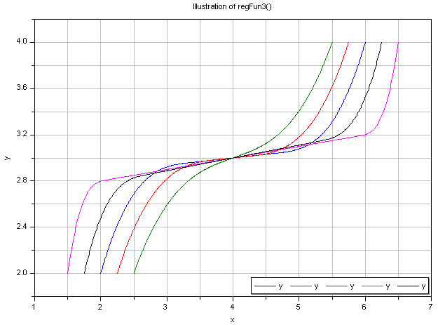
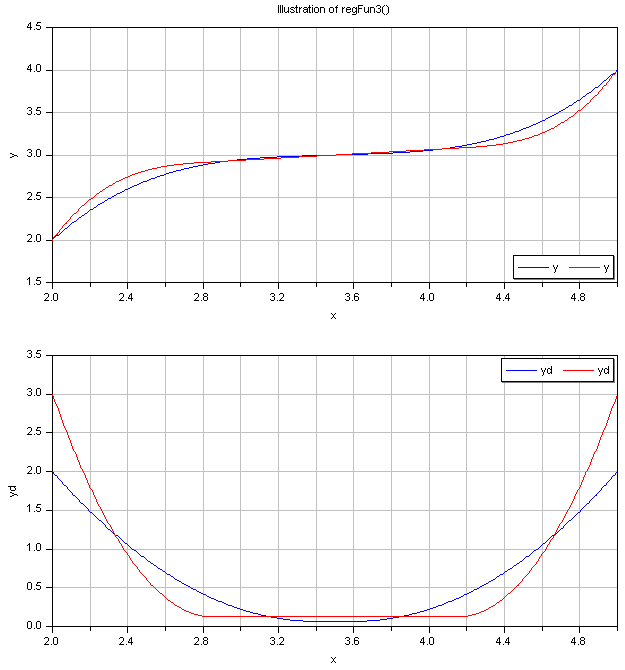
Typical screenshots for two different configurations are shown below. The first one illustrates five different settings of xi and yid:

The second graph shows the continous derivative of this regularization function:

Literature

Gasparo M. G. and Morandi R. (1991):

Piecewise cubic monotone interpolation with assigned slopes. Computing, Vol. 46, Issue 4, December 1991, pp. 355 - 365.

Inputs

Type	Name	Default	Description
Real	x		Abscissa value
Real	x0		Lower abscissa value
Real	x1		Upper abscissa value
Real	y0		Ordinate value at lower ordinate value
Real	y1		Ordinate value at upper ordinate value
Real	y0d		Derivative at lower abscissa value
Real	y1d		Derivative at upper abscissa value

Outputs

Type	Name	Description
Real	y	Ordinate value
Real	c	Slope of linear section between two cubic polynomials or dummy linear section slope if single cubic is used

Modelica definition

function regFun3 "Co-monotonic and C1 smooth regularization function"

  input Real x "Abscissa value";
  input Real x0 "Lower abscissa value";
  input Real x1 "Upper abscissa value";
  input Real y0 "Ordinate value at lower ordinate value";
  input Real y1 "Ordinate value at upper ordinate value";
  input Real y0d "Derivative at lower abscissa value";
  input Real y1d "Derivative at upper abscissa value";

  output Real y "Ordinate value";
  output Real c 
    "Slope of linear section between two cubic polynomials or dummy linear section slope if single cubic is used";

protected 
  Real h0 "Width of interval i=0";
  Real Delta0 "Slope of secant on interval i=0";
  Real xstar "Inflection point of cubic polynomial S0";
  Real mu "Distance of inflection point and left limit x0";
  Real eta "Distance of right limit x1 and inflection point";
  Real omega "Slope of subic polynomial S0 at inflection point";
  Real rho "Weighting factor of eta and eta_tilde, mu and mu_tilde";
  Real theta0 "Slope metric";
  Real mu_tilde "Distance of start of linear section and left limit x0";
  Real eta_tilde "Distance of right limit x1 and end of linear section";
  Real xi1 "Start of linear section ";
  Real xi2 "End of linear section ";
  Real a1 "Leading coefficient of cubic on the left";
  Real a2 "Leading coefficient of cubic on the right";
  Real const12 "Integration constant of left cubic, linear section";
  Real const3 "Integration constant of right cubic";
  Real aux01;
  Real aux02;
  Boolean useSingleCubicPolynomial = false 
    "Indicate to override further logic and use single cubic";
algorithm 
  assert(x0<x1, "regFun3(): Data points not sorted appropriately (x0 = "+String(x0)+" > x1 = "+String(x1)+"). Please flip arguments.");

  h0 :=x1 - x0;
  Delta0 :=(y1 - y0)/h0;

  if abs(Delta0)<=0 then
    // Points (x0,y0) and (x1,y1) on horizonzal line
    // Degenerate case as we cannot fulfill the C1 goal an comonotone behaviour at the same time
    y := y0; // == y1
  else
    // Points (x0,y0) and (x1,y1) not on horizonzal line
    if abs(y1d+y0d-2*Delta0)<100*Modelica.Constants.eps then
      xstar := (x1-x0)*(2*y0d+y1d-3*Delta0)*(if (y0d+y1d-2*Delta0)>=0 then 1 else -1)*Modelica.Constants.inf;
    else
      xstar :=1/3*(-3*x0*y0d - 3*x0*y1d + 6*x0*Delta0 - 2*h0*y0d - h0*y1d + 3*h0*
        Delta0)/(-y0d - y1d + 2*Delta0);
    end if;
    mu :=xstar - x0;
    eta :=x1 - xstar;
    omega :=3*(y0d + y1d - 2*Delta0)*(xstar - x0)^2/h0^2 + 2*(-2*y0d - y1d + 3*
      Delta0)*(xstar - x0)/h0 + y0d;

    aux01 := 0.25 * sign(Delta0) * min(abs(omega), abs(Delta0)) 
      "Slope c if not using plain cubic S0";
    if abs(y0d-y1d)<=100*Modelica.Constants.eps then
      // y0 == y1 (value and sign equal) -> resolve indefinite 0/0
      aux02 := y0d;
      if y1 > y0 + y0d*(x1-x0) then
        // If y1 is above the linear extension through (x0/y0)
        // with slope y0d (when slopes are identical)
        //  -> then always used single cubic polynomial
        useSingleCubicPolynomial := true;
      end if;
    elseif abs(y1d+y0d-2*Delta0)<100*Modelica.Constants.eps then
      // (y1d+y0d-2*Delta0) approximately 0 -> avoid division by 0
      aux02 := (6*Delta0*(y1d+y0d-3/2*Delta0)-y1d*y0d-y1d^2-y0d^2)*(if (y1d+y0d-2*Delta0)>=0 then 1 else -1)*Modelica.Constants.inf;
    else
      // Okay, no guarding necessary
      aux02 := (6*Delta0*(y1d+y0d-3/2*Delta0)-y1d*y0d-y1d^2-y0d^2)/(3*(y1d+y0d-2*Delta0));
    end if;

    //aux02 := -1/3*(y0d^2+y0d*y1d-6*y0d*Delta0+y1d^2-6*y1d*Delta0+9*Delta0^2)/(y0d+y1d-2*Delta0);
    //aux02 := -1/3*(6*y1d*y0*x1+y0d*y1d*x1^2-6*y0d*x0*y0+y0d^2*x0^2+y0d^2*x1^2+y1d^2*x1^2+y1d^2*x0^2-2*y0d*x0*y1d*x1-2*x0*y0d^2*x1+y0d*y1d*x0^2+6*y0d*x0*y1-6*y0d*y1*x1+6*y0d*y0*x1-2*x0*y1d^2*x1-6*y1d*y1*x1+6*y1d*x0*y1-6*y1d*x0*y0-18*y1*y0+9*y1^2+9*y0^2)/(y0d*x1^2-2*x0*y0d*x1+y1d*x1^2-2*x0*y1d*x1-2*y1*x1+2*y0*x1+y0d*x0^2+y1d*x0^2+2*x0*y1-2*x0*y0);

    // Test criteria (also used to avoid saddle points that lead to integrator contraction):
    //
    //  1. Cubic is not monotonic (from Gasparo Morandi)
    //       ((mu > 0) and (eta < h0) and (Delta0*omega <= 0))
    //
    //  2. Cubic may be monotonic but the linear section slope c is either too close
    //     to zero or the end point of the linear section is left of the start point
    //     Note however, that the suggested slope has to have the same sign as Delta0.
    //       (abs(aux01)<abs(aux02) and aux02*Delta0>=0)
    //
    //  3. Cubic may be monotonic but the resulting slope in the linear section
    //     is too close to zero (less than 1/10 of Delta0).
    //       (c < Delta0 / 10)
    //
    if (((mu > 0) and (eta < h0) and (Delta0*omega <= 0))
        or (abs(aux01)<abs(aux02) and aux02*Delta0>=0)
        or (abs(aux01)<abs(0.1*Delta0))) and not useSingleCubicPolynomial then
      // NOT monotonic using plain cubic S0, use piecewise function S0 tilde instead
      c := aux01;
      // Avoid saddle points that are co-monotonic but lead to integrator contraction
      if abs(c)<abs(aux02) and aux02*Delta0>=0 then
        c := aux02;
      end if;
      if abs(c)<abs(0.1*Delta0) then
        c := 0.1*Delta0;
      end if;
      theta0 := (y0d*mu + y1d*eta)/h0;
      if abs(theta0 - c)<1e-6 then
        // Slightly reduce c in order to avoid ill-posed problem
        c := (1-1e-6)*theta0;
      end if;
      rho := 3*(Delta0 - c)/(theta0 - c);
      mu_tilde := rho * mu;
      eta_tilde := rho * eta;
      xi1 := x0 + mu_tilde;
      xi2 := x1 - eta_tilde;
      a1 := (y0d - c)/max(mu_tilde^2, 100*Modelica.Constants.eps);
      a2 := (y1d - c)/max(eta_tilde^2, 100*Modelica.Constants.eps);
      const12 := y0 - a1/3*(x0 - xi1)^3 - c*x0;
      const3 := y1 - a2/3*(x1 - xi2)^3 - c*x1;
      // Do actual interpolation
      if (x < xi1) then
        y := a1/3*(x - xi1)^3 + c*x + const12;
      elseif (x < xi2) then
        y := c*x + const12;
      else
        y := a2/3*(x - xi2)^3 + c*x + const3;
      end if;
    else
      // Cubic S0 is monotonic, use it as is
      y := (y0d+y1d-2*Delta0)*(x-x0)^3/h0^2+(-2*y0d-y1d+3*Delta0)*(x-x0)^2/h0+y0d*(x-x0)+y0;
      // Provide a "dummy linear section slope" as the slope of the cubic at x:=(x0+x1)/2
      aux01 := (x0+x1)/2;
      c := 3*(y0d+y1d-2*Delta0)*(aux01-x0)^2/h0^2+2*(-2*y0d-y1d+3*Delta0)*(aux01-x0)/h0+y0d;
    end if;
  end if;

end regFun3;

Modelica.Fluid.Utilities.cubicHermite

Inputs

Type	Name	Default	Description
Real	x		Abscissa value
Real	x1		Lower abscissa value
Real	x2		Upper abscissa value
Real	y1		Lower ordinate value
Real	y2		Upper ordinate value
Real	y1d		Lower gradient
Real	y2d		Upper gradient

Outputs

Type	Name	Description
Real	y	Interpolated ordinate value

Modelica definition

function cubicHermite "Evaluate a cubic Hermite spline"
  input Real x "Abscissa value";
  input Real x1 "Lower abscissa value";
  input Real x2 "Upper abscissa value";
  input Real y1 "Lower ordinate value";
  input Real y2 "Upper ordinate value";
  input Real y1d "Lower gradient";
  input Real y2d "Upper gradient";
  output Real y "Interpolated ordinate value";
protected 
  Real h "Distance between x1 and x2";
  Real t "abscissa scaled with h, i.e., t=[0..1] within x=[x1..x2]";
  Real h00 "Basis function 00 of cubic Hermite spline";
  Real h10 "Basis function 10 of cubic Hermite spline";
  Real h01 "Basis function 01 of cubic Hermite spline";
  Real h11 "Basis function 11 of cubic Hermite spline";
  Real aux3 "t cube";
  Real aux2 "t square";
algorithm 
  h := x2 - x1;
  if abs(h)>0 then
    // Regular case
    t := (x - x1)/h;

    aux3 :=t^3;
    aux2 :=t^2;

    h00 := 2*aux3 - 3*aux2 + 1;
    h10 := aux3 - 2*aux2 + t;
    h01 := -2*aux3 + 3*aux2;
    h11 := aux3 - aux2;
    y := y1*h00 + h*y1d*h10 + y2*h01 + h*y2d*h11;
  else
    // Degenerate case, x1 and x2 are identical, return step function
    y := (y1 + y2)/2;
  end if;
end cubicHermite;

Modelica.Fluid.Utilities.cubicHermite_withDerivative

Inputs

Type	Name	Default	Description
Real	x		Abscissa value
Real	x1		Lower abscissa value
Real	x2		Upper abscissa value
Real	y1		Lower ordinate value
Real	y2		Upper ordinate value
Real	y1d		Lower gradient
Real	y2d		Upper gradient

Outputs

Type	Name	Description
Real	y	Interpolated ordinate value
Real	dy_dx	Derivative dy/dx at abscissa value x

Modelica definition

function cubicHermite_withDerivative 
  "Evaluate a cubic Hermite spline, return value and derivative"
  input Real x "Abscissa value";
  input Real x1 "Lower abscissa value";
  input Real x2 "Upper abscissa value";
  input Real y1 "Lower ordinate value";
  input Real y2 "Upper ordinate value";
  input Real y1d "Lower gradient";
  input Real y2d "Upper gradient";
  output Real y "Interpolated ordinate value";
  output Real dy_dx "Derivative dy/dx at abscissa value x";
protected 
  Real h "Distance between x1 and x2";
  Real t "abscissa scaled with h, i.e., t=[0..1] within x=[x1..x2]";
  Real h00 "Basis function 00 of cubic Hermite spline";
  Real h10 "Basis function 10 of cubic Hermite spline";
  Real h01 "Basis function 01 of cubic Hermite spline";
  Real h11 "Basis function 11 of cubic Hermite spline";

  Real h00d "d/dt h00";
  Real h10d "d/dt h10";
  Real h01d "d/dt h01";
  Real h11d "d/dt h11";

  Real aux3 "t cube";
  Real aux2 "t square";
algorithm 
  h := x2 - x1;
  if abs(h)>0 then
    // Regular case
    t := (x - x1)/h;

    aux3 :=t^3;
    aux2 :=t^2;

    h00 := 2*aux3 - 3*aux2 + 1;
    h10 := aux3 - 2*aux2 + t;
    h01 := -2*aux3 + 3*aux2;
    h11 := aux3 - aux2;

    h00d := 6*(aux2 - t);
    h10d := 3*aux2 - 4*t + 1;
    h01d := 6*(t - aux2);
    h11d := 3*aux2 - 2*t;

    y := y1*h00 + h*y1d*h10 + y2*h01 + h*y2d*h11;
    dy_dx := y1*h00d/h + y1d*h10d + y2*h01d/h + y2d*h11d;
  else
    // Degenerate case, x1 and x2 are identical, return step function
    y := (y1 + y2)/2;
    dy_dx := sign(y2 - y1)*Modelica.Constants.inf;
  end if;
end cubicHermite_withDerivative;