Buildings.Fluid.HydronicConfigurations.ActiveNetworks.Examples
Example models
Information
This package contains examples for the use of models that can be found in Buildings.Fluid.HydronicConfigurations.ActiveNetworks.
Extends from Modelica.Icons.ExamplesPackage (Icon for packages containing runnable examples).
Package Content
| Name | Description |
|---|---|
| Model illustrating the operation of a decoupling circuit | |
| Model illustrating the operation of a decoupling circuit serving a single mixing circuit | |
| Model illustrating the operation of a decoupling circuit with Delta-T control | |
| Model illustrating the operation of diversion circuits with constant speed pump | |
| Model illustrating the operation of an inversion circuit with three-way valve | |
| Model illustrating the operation of an inversion circuit with two-way valve and check valve and variable secondary | |
| Model illustrating the operation of an inversion circuit with two-way valve and constant secondary | |
| Model illustrating the operation of an inversion circuit with two-way valve and variable secondary | |
| Model illustrating the operation of an inversion circuit with two-way valve and variable secondary with return temperature control | |
| Model illustrating the operation of single mixing circuits | |
| Model illustrating the operation of throttle circuits with variable speed pump | |
| Package with base classes |
 Buildings.Fluid.HydronicConfigurations.ActiveNetworks.Examples.Decoupling
Model illustrating the operation of a decoupling circuit
Information
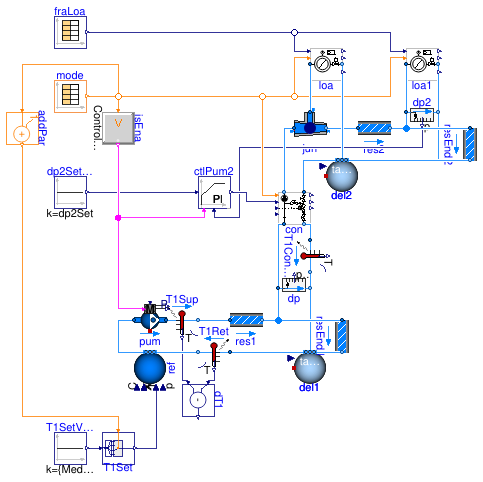
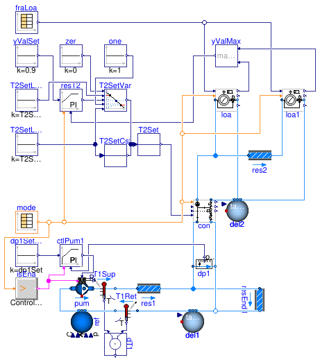
This model represents a change-over system where the configuration Buildings.Fluid.HydronicConfigurations.ActiveNetworks.Decoupling serves as the interface between a variable flow primary circuit and a variable flow consumer circuit operated in change-over. For a given operating mode, both the primary circuit and the consumer circuit have a constant supply temperature.
The model illustrates how the primary flow rate varies with the secondary flow rate, yielding a nearly constant bypass mass flow rate.
Extends from BaseClasses.PartialDecoupling (Partial model of primary variable circuit serving a decoupling circuit).
Parameters
| Type | Name | Default | Description |
|---|---|---|---|
| Control | typ | Buildings.Fluid.HydronicConf... | Load type |
| Integer | nTer | 2 | Number of terminal units |
| Real | kSizPum | 1.0 | Pump oversizing coefficient [1] |
| Pressure | p_min | 200000 | Circuit minimum pressure [Pa] |
| Temperature | TLiqEnt_nominal | if typ == Buildings.Fluid.Hy... | Liquid entering temperature at design conditions [K] |
| Temperature | TLiqLvg_nominal | TLiqEnt_nominal + (if typ ==... | Liquid leaving temperature at design conditions [K] |
| Temperature | TLiqEntChg_nominal | 60 + 273.15 | Liquid entering temperature in change-over mode [K] |
| Temperature | TLiqSup_nominal | TLiqEnt_nominal | Liquid primary supply temperature at design conditions [K] |
| Temperature | TLiqSupChg_nominal | TLiqEntChg_nominal | Liquid primary supply temperature in change-over mode [K] |
| PressureDifference | dp1_nominal | dpPum_nominal - dpPip_nominal | Control valve pressure drop at design conditions [Pa] |
| Nominal condition | |||
| MassFlowRate | mTer_flow_nominal | 1 | Terminal unit mass flow rate at design conditions [kg/s] |
| MassFlowRate | m1_flow_nominal | 1.1*m2_flow_nominal | Mass flow rate in primary branch at design conditions [kg/s] |
| MassFlowRate | m2_flow_nominal | nTer*mTer_flow_nominal/0.9 | Mass flow rate in consumer circuit at design conditions [kg/s] |
| PressureDifference | dpTer_nominal | 3E4 | Terminal unit pressure drop at design conditions [Pa] |
| PressureDifference | dpPip_nominal | 0.5E4 | Pipe section pressure drop at design conditions [Pa] |
| PressureDifference | dpPum_nominal | 10e4 | Pump head at design conditions [Pa] |
| MassFlowRate | mPum_flow_nominal | m1_flow_nominal/0.9 | Primary pump mass flow rate at design conditions [kg/s] |
| PressureDifference | dp2_nominal | dpPip_nominal + dp2Set | Consumer circuit pressure differential at design conditions [Pa] |
| Configuration | |||
| Boolean | is_bal | true | Set to true for balanced primary branch |
| Controls | |||
| PressureDifference | dp2Set | loa1.dpTer_nominal + loa1.dp... | Consumer circuit pressure differential set point [Pa] |
| Dynamics | |||
| Conservation equations | |||
| Dynamics | energyDynamics | Modelica.Fluid.Types.Dynamic... | Type of energy balance: dynamic (3 initialization options) or steady state |
Modelica definition
Buildings.Fluid.HydronicConfigurations.ActiveNetworks.Examples.DecouplingMixing
Model illustrating the operation of a decoupling circuit serving a single mixing circuit
Information
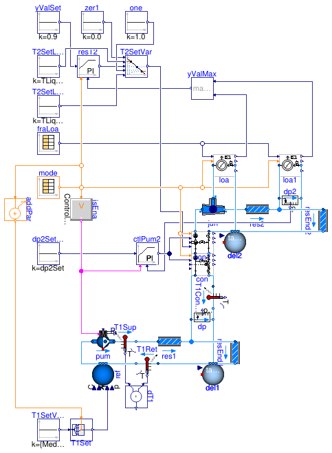
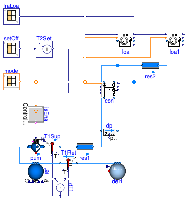
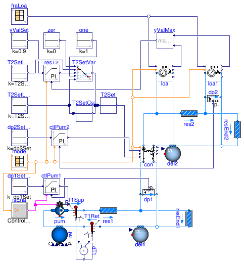
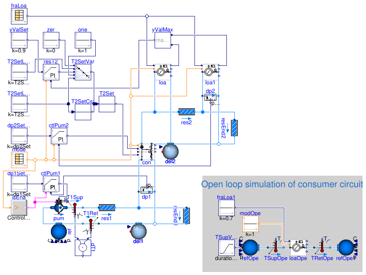
This model represents a cooling system where the configuration Buildings.Fluid.HydronicConfigurations.ActiveNetworks.Decoupling is used in conjunction with Buildings.Fluid.HydronicConfigurations.PassiveNetworks.SingleMixing. The combined configuration serves as the interface between a variable flow primary circuit and a variable flow consumer circuit. The primary circuit has a constant supply temperature. The consumer circuit has a varying supply temperature set point that is reset based on the terminal valve opening, with the most open valve being kept 90% open.
Note the following settings.
-
con1.dp1_nominal=con.dpBal3_nominalwhich is used to size the control valve and the pump of the mixing configuration, and avoids a reverse flow in the bypass at partial load due to the opposing differential pressure created by the decoupling configuration. See Buildings.Fluid.HydronicConfigurations.PassiveNetworks.Examples.SingleMixingOpenLoop for further details on that behavior. -
The controller
resT2that is used to reset the secondary supply temperature usesy_reset=1which yields the design supply temperature at the time when the controller is enabled. Otherwise there is a significant delay in satisfying the load, followed by a large overshoot, and the control loop is hard to tune.
The fact that the load seems unmet at partial load (see plot #4) is due to the load model that does not guarantee a linear variation of the load with the input signal in cooling mode, see Buildings.Fluid.HydronicConfigurations.ActiveNetworks.Examples.BaseClasses.Load.
Extends from Buildings.Fluid.HydronicConfigurations.ActiveNetworks.Examples.BaseClasses.PartialDecoupling (Partial model of primary variable circuit serving a decoupling circuit).
Parameters
| Type | Name | Default | Description |
|---|---|---|---|
| Control | typ | Buildings.Fluid.HydronicConf... | Load type |
| Integer | nTer | 2 | Number of terminal units |
| Real | kSizPum | 1.0 | Pump oversizing coefficient [1] |
| Pressure | p_min | 200000 | Circuit minimum pressure [Pa] |
| Temperature | TLiqEnt_nominal | if typ == Buildings.Fluid.Hy... | Liquid entering temperature at design conditions [K] |
| Temperature | TLiqLvg_nominal | TLiqEnt_nominal + (if typ ==... | Liquid leaving temperature at design conditions [K] |
| Temperature | TLiqEntChg_nominal | 60 + 273.15 | Liquid entering temperature in change-over mode [K] |
| Temperature | TLiqSup_nominal | TLiqEnt_nominal | Liquid primary supply temperature at design conditions [K] |
| Temperature | TLiqSupChg_nominal | TLiqEntChg_nominal | Liquid primary supply temperature in change-over mode [K] |
| PressureDifference | dp1_nominal | dpPum_nominal - dpPip_nominal | Control valve pressure drop at design conditions [Pa] |
| Nominal condition | |||
| MassFlowRate | mTer_flow_nominal | 1 | Terminal unit mass flow rate at design conditions [kg/s] |
| MassFlowRate | m1_flow_nominal | 1.1*m2_flow_nominal | Mass flow rate in primary branch at design conditions [kg/s] |
| MassFlowRate | m2_flow_nominal | nTer*mTer_flow_nominal/0.9 | Mass flow rate in consumer circuit at design conditions [kg/s] |
| PressureDifference | dpTer_nominal | 3E4 | Terminal unit pressure drop at design conditions [Pa] |
| PressureDifference | dpPip_nominal | 0.5E4 | Pipe section pressure drop at design conditions [Pa] |
| PressureDifference | dpPum_nominal | 10e4 | Pump head at design conditions [Pa] |
| MassFlowRate | mPum_flow_nominal | m1_flow_nominal/0.9 | Primary pump mass flow rate at design conditions [kg/s] |
| PressureDifference | dp2_nominal | dpPip_nominal + dp2Set | Consumer circuit pressure differential at design conditions [Pa] |
| Configuration | |||
| Boolean | is_bal | true | Set to true for balanced primary branch |
| Controls | |||
| PressureDifference | dp2Set | loa1.dpTer_nominal + loa1.dp... | Consumer circuit pressure differential set point [Pa] |
| Dynamics | |||
| Conservation equations | |||
| Dynamics | energyDynamics | Modelica.Fluid.Types.Dynamic... | Type of energy balance: dynamic (3 initialization options) or steady state |
Modelica definition
Buildings.Fluid.HydronicConfigurations.ActiveNetworks.Examples.DecouplingTemperature
Model illustrating the operation of a decoupling circuit with Delta-T control
Information
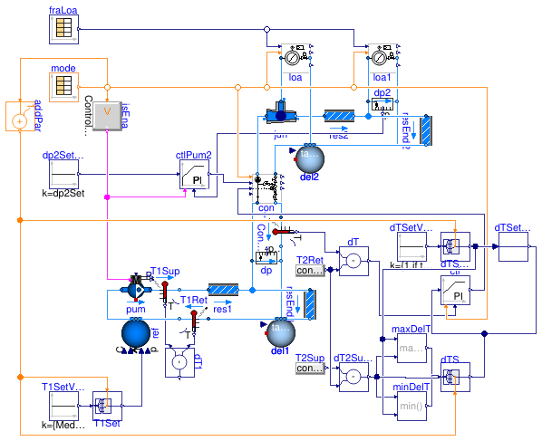
This example is similar to Buildings.Fluid.HydronicConfigurations.ActiveNetworks.Examples.Decoupling except that an alternative control logic is implemented, based on the measurement of the return temperature in the consumer circuit and in the primary branch.
This control logic intends to keep constant the difference between those two
measurements.
Considering that we have:
T1, ret - T2, ret =
(ṁ1 - ṁ2) / ṁ1 *
(T1, sup - T2, ret),
the control objective can be expressed based on the
set point ΔTset and the consumer circuit
temperature differential ΔT2
(ΔT2 = T2, sup - T2, ret =
T1, sup - T2, ret)
as:
ΔTset =
(ṁ1 - ṁ2) / ṁ1 *
ΔT2.
For consumer circuits that have a temperature differential
relatively constant (see for instance
Buildings.Fluid.HydronicConfigurations.ActiveNetworks.Examples.ThrottleOpenLoop),
the control logic will thus maintain a
nearly constant fraction of primary flow recirculation.
However, at very low load if ΔT2 value
drops (due for instance to a secondary flow recirculation
ensuring a minimum flow for the secondary pump) the
control valve will be fully open, and the primary pump speed
potentially maxed out, trying to compensate for the vanishing
ΔT2.
In other words, taking the example of a heating circuit, at low
load the control logic cannot infer that the low
value of T1, ret - T2, ret is due
to a consumer circuit return temperature that is too high
(as it tends towards the supply temperature).
It will work under the assumption that T1, ret
is too low, and open the control valve to try and increase the
primary flow recirculation.
This flawed control is showcased in this example when the parameter
is_cor is set to false (the default), see
plots #1 and #2 between 14 and 16 h.
Now setting is_cor to true, a correction
is used to counteract this low load effect
by limiting the set point to the consumer circuit temperature differential
ΔT2.
Note that the implementation of that correction is specific to
a change-over operation and needs to be adapted for heating-only
or cooling-only applications.
Extends from Buildings.Fluid.HydronicConfigurations.ActiveNetworks.Examples.Decoupling (Model illustrating the operation of a decoupling circuit).
Parameters
| Type | Name | Default | Description |
|---|---|---|---|
| Control | typ | Buildings.Fluid.HydronicConf... | Load type |
| Integer | nTer | 2 | Number of terminal units |
| Real | kSizPum | 1.0 | Pump oversizing coefficient [1] |
| Pressure | p_min | 200000 | Circuit minimum pressure [Pa] |
| Temperature | TLiqEnt_nominal | if typ == Buildings.Fluid.Hy... | Liquid entering temperature at design conditions [K] |
| Temperature | TLiqLvg_nominal | TLiqEnt_nominal + (if typ ==... | Liquid leaving temperature at design conditions [K] |
| Temperature | TLiqEntChg_nominal | 60 + 273.15 | Liquid entering temperature in change-over mode [K] |
| Temperature | TLiqSup_nominal | TLiqEnt_nominal | Liquid primary supply temperature at design conditions [K] |
| Temperature | TLiqSupChg_nominal | TLiqEntChg_nominal | Liquid primary supply temperature in change-over mode [K] |
| PressureDifference | dp1_nominal | dpPum_nominal - dpPip_nominal | Control valve pressure drop at design conditions [Pa] |
| Boolean | is_cor | false | Set to true to correct Delta-T set point for low load operation |
| Nominal condition | |||
| MassFlowRate | mTer_flow_nominal | 1 | Terminal unit mass flow rate at design conditions [kg/s] |
| MassFlowRate | m1_flow_nominal | 1.1*m2_flow_nominal | Mass flow rate in primary branch at design conditions [kg/s] |
| MassFlowRate | m2_flow_nominal | nTer*mTer_flow_nominal/0.9 | Mass flow rate in consumer circuit at design conditions [kg/s] |
| PressureDifference | dpTer_nominal | 3E4 | Terminal unit pressure drop at design conditions [Pa] |
| PressureDifference | dpPip_nominal | 0.5E4 | Pipe section pressure drop at design conditions [Pa] |
| PressureDifference | dpPum_nominal | 10e4 | Pump head at design conditions [Pa] |
| MassFlowRate | mPum_flow_nominal | m1_flow_nominal/0.9 | Primary pump mass flow rate at design conditions [kg/s] |
| PressureDifference | dp2_nominal | dpPip_nominal + dp2Set | Consumer circuit pressure differential at design conditions [Pa] |
| Configuration | |||
| Boolean | is_bal | true | Set to true for balanced primary branch |
| Controls | |||
| PressureDifference | dp2Set | loa1.dpTer_nominal + loa1.dp... | Consumer circuit pressure differential set point [Pa] |
| Dynamics | |||
| Conservation equations | |||
| Dynamics | energyDynamics | Modelica.Fluid.Types.Dynamic... | Type of energy balance: dynamic (3 initialization options) or steady state |
Modelica definition
Buildings.Fluid.HydronicConfigurations.ActiveNetworks.Examples.DiversionOpenLoop
Model illustrating the operation of diversion circuits with constant speed pump
Information
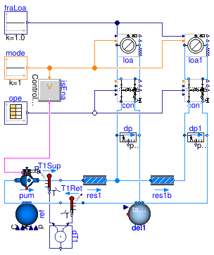
This model represents a heating system where the configuration Buildings.Fluid.HydronicConfigurations.ActiveNetworks.Diversion is used to modulate the heat flow rate transmitted to a constant load. Two identical secondary circuits are connected to a primary circuit with a constant speed pump. The main assumptions are enumerated below.
- The model is configured in steady-state.
-
The design conditions at
time=0are defined without considering any load diversity. - Each circuit is balanced at design conditions.
-
The bypass of the diversion circuit is balanced at
design conditions if the parameter
is_balis set totrue. Otherwise no fixed flow resistance is considered in the bypass branch, only the variable flow resistance corresponding to the bypass port of the three-way valve.
When simulated with the default parameter values, this example shows the following points.
-
The overflow caused by the unbalanced bypass when the valve
is fully closed in the first circuit (see plot #2 at
time=100) creates a concomitant flow shortage in the second circuit with the valve fully open. However, the flow shortage (4%) is of a much lower amplitude than the overflow (30%). Indeed the equivalent flow resistance seen by the pump is lower than at design conditions, leading a shift of the operating point of the pump towards a flow rate value higher than design, which partly compensates for the overflow. - The impact on the heat flow rate transferred to the load (see plot #4) is of an even lower amplitude (2%). This is dependent on the emission characteristic of the terminal unit that would theoretically be steeper with a higher effectiveness at design conditions, although the order of magnitude would remain the same. For reference, the terminal unit in this example represents a recirculating air terminal such as a fan coil unit in heating mode with a water ΔT of 10 °C at design conditions, so an effectiveness ε = ΔTliq / (Tliq, inl - Tair, inl) = 0.25.
- The equal-percentage / linear characteristic of the control valve yields a relationship between the heat flow rate transferred to the load and the valve opening that is close to linear (see plot #4), with a Pearson correlation coefficient equal to 0.99.
Sensitivity analysis
Those observations are confirmed by a sensitivity study to the following parameters.
- Ratio of the terminal unit pressure drop to the pump head at design conditions (refer to the schematic in the documentation of Buildings.Fluid.HydronicConfigurations.ActiveNetworks.Diversion for the nomenclature): ψ = ΔpJ-A / Δppump varying from 0.1 to 0.4
- Ratio of the control valve authority: β = ΔpA-AB / ΔpJ-AB varying from 0.1 to 0.7
-
Balanced bypass branch:
is_balswitched fromfalsetotrue -
Valve characteristic:
ThreeWayValveswitched from equal percentage-linear (EL) to linear-linear (LL).
Direct and bypass mass flow rate
The overflow in the bypass branch when the valve is fully closed increases with ψ and decreases with β. It is close to 70% for ψ = 40% and β = 10%. However, the concomitant flow shortage in the other terminal unit with a valve fully open (see Figure 2) is limited to 12%. For a valve authority of β = 50% one may note that the flow shortage is below 5%, indicating that selecting the control valve with a suitable authority largely dampens the impact of an unbalanced bypass.
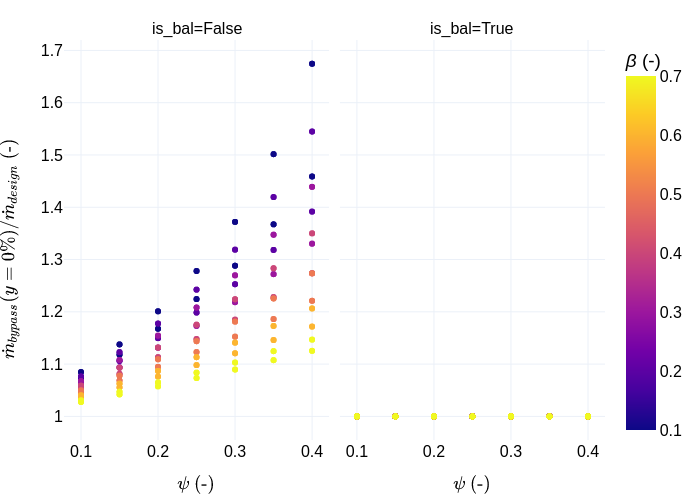
Figure 1. Bypass mass flow rate (ratio to design value) at fully closed conditions
as a function of
ψ for various valve authorities β (color scale),
and a bypass branch either balanced (right plot) or not (left plot).
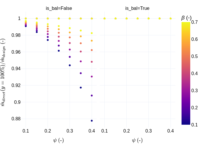
Figure 2. Direct mass flow rate (ratio to design value) at fully open conditions
as a function of
ψ for various valve authorities β (color scale),
and a bypass branch either balanced (right plot) or not (left plot).
Primary mass flow rate
The total primary mass flow rate (or pump mass flow rate) is plotted on Figure 3. This helps assess the actual flow variation in "constant flow circuits", i.e., constant speed pump distribution systems with terminal units equipped with three-way control valves. The total pump flow can vary up to 50% when the bypass of the three-way valves is not balanced, whereas the flow variation is limited to about 20% when the bypass of the three-way valves is balanced. If the characteristic of the valves is equal percentage and linear, this variation is rather by higher values for an unbalanced bypass and by lower values for a balanced bypass. If the characteristic of the valves is linear and linear, this variation is always by higher values. Eventually, when the control valve authority is higher than 0.5 the flow variation is limited to about ±20% in all cases.
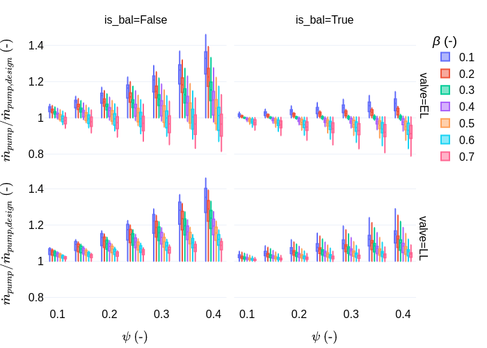
Figure 3. Pump mass flow rate (ratio to design value) as a function of
ψ for various valve authorities β (color scale),
a bypass branch either balanced (right plots) or not (left plots)
and either an equal-percentage / linear valve characteristic (top plots)
or a linear / linear valve characteristic (bottom plots).
Heat flow rate transferred to the load
The heat flow rate transferred to the load is presented
- on Figure 4 at full opening to illustrate the impact on the coil capacity of the flow shortage previously discussed,
- on Figure 5 at 10% opening to illustrate the linearity of the relationship between the transmitted heat flow rate and the valve opening at low load in the case of an equal percentage valve (where values of the heat flow rate close to 10% of the coil capacity indicate a good linearity).
The impact on the coil capacity of the flow shortage due to an unbalanced bypass is limited to about 5% and is less than 2% for an authority higher or equal to 0.5. A balanced bypass tends to disturb the linearity of the heat flow rate with the valve opening. But again, if the valve is selected with an authority higher or equal to 0.5 that disturbance is highly reduced.
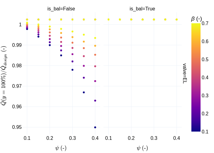
Figure 4. Heat flow rate (ratio to design value) at fully open conditions
as a function of
ψ for various valve authorities β (color scale),
and a bypass branch either balanced (right plot) or not (left plot).
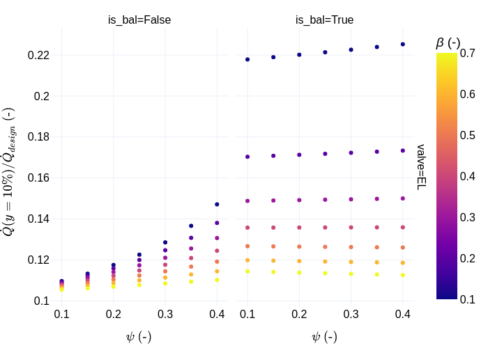
Figure 5. Heat flow rate (ratio to design value) at 10% open conditions
as a function of ψ for various valve authorities β (color scale),
and a bypass branch either balanced (right plot) or not (left plot).
Extends from BaseClasses.PartialActivePrimary (Partial model of active primary network).
Parameters
| Type | Name | Default | Description |
|---|---|---|---|
| Control | typ | Buildings.Fluid.HydronicConf... | Load type |
| Integer | nTer | 2 | Number of terminal units |
| Real | kSizPum | 1.0 | Pump oversizing coefficient [1] |
| Pressure | p_min | 200000 | Circuit minimum pressure [Pa] |
| Temperature | TLiqEnt_nominal | if typ == Buildings.Fluid.Hy... | Liquid entering temperature at design conditions [K] |
| Temperature | TLiqLvg_nominal | TLiqEnt_nominal + (if typ ==... | Liquid leaving temperature at design conditions [K] |
| Temperature | TLiqEntChg_nominal | 60 + 273.15 | Liquid entering temperature in change-over mode [K] |
| Temperature | TLiqSup_nominal | TLiqEnt_nominal | Liquid primary supply temperature at design conditions [K] |
| Temperature | TLiqSupChg_nominal | TLiqEntChg_nominal | Liquid primary supply temperature in change-over mode [K] |
| PressureDifference | dpValve_nominal | dpTer_nominal | Control valve pressure drop at design conditions [Pa] |
| Nominal condition | |||
| MassFlowRate | mTer_flow_nominal | 1 | Terminal unit mass flow rate at design conditions [kg/s] |
| MassFlowRate | m1_flow_nominal | m2_flow_nominal | Mass flow rate in primary branch at design conditions [kg/s] |
| MassFlowRate | m2_flow_nominal | nTer*mTer_flow_nominal | Mass flow rate in consumer circuit at design conditions [kg/s] |
| PressureDifference | dpTer_nominal | 3E4 | Terminal unit pressure drop at design conditions [Pa] |
| PressureDifference | dpPip_nominal | 0.5E4 | Pipe section pressure drop at design conditions [Pa] |
| PressureDifference | dpPum_nominal | (2*dpPip_nominal + dpTer_nom... | Pump head at design conditions [Pa] |
| MassFlowRate | mPum_flow_nominal | m1_flow_nominal | Primary pump mass flow rate at design conditions [kg/s] |
| PressureDifference | dpBal3_nominal | if is_bal then dpTer_nominal... | Bypass balancing valve pressure drop at design conditions [Pa] |
| Configuration | |||
| Boolean | is_bal | false | Set to true for a balanced bypass |
| ValveCharacteristic | typCha | Buildings.Fluid.HydronicConf... | Control valve characteristic |
| Dynamics | |||
| Conservation equations | |||
| Dynamics | energyDynamics | Modelica.Fluid.Types.Dynamic... | Type of energy balance: dynamic (3 initialization options) or steady state |
Modelica definition
Buildings.Fluid.HydronicConfigurations.ActiveNetworks.Examples.InjectionThreeWay
Model illustrating the operation of an inversion circuit with three-way valve
Information
This model represents a heating system where the configuration Buildings.Fluid.HydronicConfigurations.ActiveNetworks.InjectionThreeWay serves as the interface between a constant flow primary circuit at constant supply temperature and a constant flow secondary circuit at variable supply temperature. The secondary supply temperature is reset with an open loop, representing for instance a reset logic based on the outdoor air temperature. Two identical terminal units are served by the secondary circuit. Each terminal unit has its own hourly load profile.
The primary side of the injection circuit is balanced at design conditions
if kSizBal=1.
Selecting a lower value of the parameter kSizBal illustrates
the operation with an oversized balancing valve, yielding
a lower pressure drop.
One can observe the degraded ΔT (plot #6) and elevated mass flow rate
(plot #7) in the primary circuit.
However, the operation of the consumer circuit is not disturbed:
the set point and the loads are met.
Extends from BaseClasses.PartialActivePrimary (Partial model of active primary network).
Parameters
| Type | Name | Default | Description |
|---|---|---|---|
| Control | typ | Buildings.Fluid.HydronicConf... | Load type |
| Integer | nTer | 2 | Number of terminal units |
| Real | kSizPum | 5.0 | Pump oversizing coefficient [1] |
| Pressure | p_min | 200000 | Circuit minimum pressure [Pa] |
| Temperature | TLiqEnt_nominal | 40 + 273.15 | Liquid entering temperature at design conditions [K] |
| Temperature | TLiqLvg_nominal | TLiqEnt_nominal - 5 | Liquid leaving temperature at design conditions [K] |
| Temperature | TLiqEntChg_nominal | 60 + 273.15 | Liquid entering temperature in change-over mode [K] |
| Temperature | TLiqSup_nominal | 60 + 273.15 | Liquid primary supply temperature at design conditions [K] |
| Temperature | TLiqSupChg_nominal | TLiqEntChg_nominal | Liquid primary supply temperature in change-over mode [K] |
| Nominal condition | |||
| MassFlowRate | mTer_flow_nominal | 1 | Terminal unit mass flow rate at design conditions [kg/s] |
| MassFlowRate | m1_flow_nominal | m2_flow_nominal*(TLiqEnt_nom... | Mass flow rate in primary branch at design conditions [kg/s] |
| MassFlowRate | m2_flow_nominal | nTer*mTer_flow_nominal | Mass flow rate in consumer circuit at design conditions [kg/s] |
| PressureDifference | dpTer_nominal | 3E4 | Terminal unit pressure drop at design conditions [Pa] |
| PressureDifference | dpPip_nominal | 0.5E4 | Pipe section pressure drop at design conditions [Pa] |
| PressureDifference | dpPum_nominal | (dpPip_nominal + con.dpValve... | Pump head at design conditions [Pa] |
| MassFlowRate | mPum_flow_nominal | m1_flow_nominal | Primary pump mass flow rate at design conditions [kg/s] |
| Configuration | |||
| Real | kSizBal | 0.5 | Sizing factor for primary balancing valve (1 means balanced) |
| Dynamics | |||
| Conservation equations | |||
| Dynamics | energyDynamics | Modelica.Fluid.Types.Dynamic... | Type of energy balance: dynamic (3 initialization options) or steady state |
Modelica definition
Buildings.Fluid.HydronicConfigurations.ActiveNetworks.Examples.InjectionTwoWayCheckValve
Model illustrating the operation of an inversion circuit with two-way valve and check valve and variable secondary
Information
This model is nearly similar to Buildings.Fluid.HydronicConfigurations.ActiveNetworks.Examples.InjectionTwoWayVariable except that
- Buildings.Fluid.HydronicConfigurations.ActiveNetworks.InjectionTwoWayCheckValve is used to connect the consumer circuit in place of Buildings.Fluid.HydronicConfigurations.ActiveNetworks.InjectionTwoWay,
- the consumer circuit set point is modified, together with the gain and the time constant of the PI controller to simulate a loose control and trigger the check valve closing at around 8 h in model time.
Extends from InjectionTwoWayVariable (Model illustrating the operation of an inversion circuit with two-way valve and variable secondary).
Parameters
| Type | Name | Default | Description |
|---|---|---|---|
| Control | typ | Buildings.Fluid.HydronicConf... | Load type |
| Integer | nTer | 2 | Number of terminal units |
| Real | kSizPum | 1.0 | Pump oversizing coefficient [1] |
| Pressure | p_min | 200000 | Circuit minimum pressure [Pa] |
| Temperature | TLiqEnt_nominal | 277.55 | Liquid entering temperature at design conditions [K] |
| Temperature | TLiqLvg_nominal | 286.65 | Liquid leaving temperature at design conditions [K] |
| Temperature | TLiqEntChg_nominal | 60 + 273.15 | Liquid entering temperature in change-over mode [K] |
| Temperature | TLiqSup_nominal | 276.15 | Liquid primary supply temperature at design conditions [K] |
| Temperature | TLiqSupChg_nominal | TLiqEntChg_nominal | Liquid primary supply temperature in change-over mode [K] |
| Nominal condition | |||
| MassFlowRate | mTer_flow_nominal | 2.46 | Terminal unit mass flow rate at design conditions [kg/s] |
| MassFlowRate | m1_flow_nominal | m2_flow_nominal*(TLiqEnt_nom... | Mass flow rate in primary branch at design conditions [kg/s] |
| MassFlowRate | m2_flow_nominal | 2*mTer_flow_nominal/0.9 | Mass flow rate in consumer circuit at design conditions [kg/s] |
| PressureDifference | dpTer_nominal | 3E4 | Terminal unit pressure drop at design conditions [Pa] |
| PressureDifference | dpPip_nominal | 0.5E4 | Pipe section pressure drop at design conditions [Pa] |
| PressureDifference | dpPum_nominal | (dpPip_nominal + dp1Set)*kSi... | Pump head at design conditions [Pa] |
| MassFlowRate | mPum_flow_nominal | m1_flow_nominal/0.9 | Primary pump mass flow rate at design conditions [kg/s] |
| PressureDifference | dp2_nominal | dpPip_nominal + dp2Set | Consumer circuit pressure differential at design conditions [Pa] |
| Temperature | T2Set_nominal | 3.2 + 273.15 | Consumer circuit design temperature set point [K] |
| Temperature | TAirEnt_nominal | 298.75 | Air entering temperature at design conditions [K] |
| MassFraction | phiAirEnt_nominal | 0.5 | Air entering relative humidity at design conditions [1] |
| MassFlowRate | mAir_flow_nominal | 6.8 | Air mass flow rate at design conditions [kg/s] |
| Configuration | |||
| Boolean | is_bal | false | Set to true for balanced primary branch |
| Boolean | have_resT2 | false | Set to true for consumer circuit temperature reset, false for constant set point |
| Controls | |||
| PressureDifference | dp1Set | 1e4 | Pressure differential set point [Pa] |
| PressureDifference | dp2Set | loa1.dpTer_nominal + loa1.dp... | Secondary pressure differential set point [Pa] |
| Dynamics | |||
| Conservation equations | |||
| Dynamics | energyDynamics | Modelica.Fluid.Types.Dynamic... | Type of energy balance: dynamic (3 initialization options) or steady state |
Modelica definition
Buildings.Fluid.HydronicConfigurations.ActiveNetworks.Examples.InjectionTwoWayConstant
Model illustrating the operation of an inversion circuit with two-way valve and constant secondary
Information
This model represents a heating system where the configuration Buildings.Fluid.HydronicConfigurations.ActiveNetworks.InjectionTwoWay serves as the interface between a variable flow primary circuit and a constant flow secondary circuit. Two identical terminal units are served by the secondary circuit. Each terminal unit has its own hourly load profile. The main assumptions are enumerated below.
- The design conditions are defined without considering any load diversity.
- Each circuit is balanced at design conditions.
- The pump dissipated heat is not added to the fluid.
-
The consumer circuit has either a constant (supply or return)
temperature set point if
have_resT2=falseor a temperature reset ifhave_resT2=true. The reset logic is based on the terminal valve opening, with the most open valve being kept 90% open.
Without temperature reset (have_resT2=false),
the primary flow variation with the load is not optimal (see plot #8):
for a load fraction of 30% the normalized primary flow rate
is about 60%.
The flow reduction is enhanced when using a reset based on the maximum
valve demand:
for a load fraction of 30% the normalized primary flow rate
is now close to 30%.
(Also note the setting of the controller resT2 which ensures
a reset at design value when the control loop is enabled).
The flow reduction is further enhanced when using a control based on the
return temperature
(have_resT2 = false and
con(typVar=Types.ControlVariable.ReturnTemperature)):
the normalized primary flow rate varies close to linearly with the
load fraction.
This explains why this control strategy is often adopted
as it brings a good flow rate variation with the load at a
first cost lower than the previous reset option based on the valve demand.
However, it also brings some additional constraints on the sizing of
the terminal units.
The load diversity must indeed be accounted for.
When tracking the return temperature of a constant flow consumer circuit,
the supply temperature will vary with the aggregated load.
In our example, the actual value of the secondary supply temperature
is lower than its design value at partial load, which yields unmet loads
(see plot #4). The terminal units should be sized accordingly,
based on the lowest possible ΔT when one terminal unit may still be at peak load.
Additional caveats speak against the use of return temperature control
with this hydronic configuration in the case of variable flow consumer circuits,
see
Buildings.Fluid.HydronicConfigurations.ActiveNetworks.Examples.InjectionTwoWayVariableReturn.
Extends from Fluid.HydronicConfigurations.ActiveNetworks.Examples.BaseClasses.PartialInjectionTwoWay (Partial model of primary variable circuit serving an inversion circuit with two-way valve).
Parameters
| Type | Name | Default | Description |
|---|---|---|---|
| Control | typ | Buildings.Fluid.HydronicConf... | Load type |
| Integer | nTer | 2 | Number of terminal units |
| Real | kSizPum | 1.0 | Pump oversizing coefficient [1] |
| Pressure | p_min | 200000 | Circuit minimum pressure [Pa] |
| Temperature | TLiqEnt_nominal | 55 + 273.15 | Liquid entering temperature at design conditions [K] |
| Temperature | TLiqLvg_nominal | TLiqEnt_nominal + (if typ ==... | Liquid leaving temperature at design conditions [K] |
| Temperature | TLiqEntChg_nominal | 60 + 273.15 | Liquid entering temperature in change-over mode [K] |
| Temperature | TLiqSup_nominal | 60 + 273.15 | Liquid primary supply temperature at design conditions [K] |
| Temperature | TLiqSupChg_nominal | TLiqEntChg_nominal | Liquid primary supply temperature in change-over mode [K] |
| LoadThreeWayValveControl | loa | redeclare BaseClasses.LoadTh... | Load |
| LoadThreeWayValveControl | loa1 | redeclare BaseClasses.LoadTh... | Load |
| Nominal condition | |||
| MassFlowRate | mTer_flow_nominal | 1 | Terminal unit mass flow rate at design conditions [kg/s] |
| MassFlowRate | m1_flow_nominal | m2_flow_nominal*(TLiqEnt_nom... | Mass flow rate in primary branch at design conditions [kg/s] |
| MassFlowRate | m2_flow_nominal | nTer*mTer_flow_nominal | Mass flow rate in consumer circuit at design conditions [kg/s] |
| PressureDifference | dpTer_nominal | 3E4 | Terminal unit pressure drop at design conditions [Pa] |
| PressureDifference | dpPip_nominal | 0.5E4 | Pipe section pressure drop at design conditions [Pa] |
| PressureDifference | dpPum_nominal | (dpPip_nominal + dp1Set)*kSi... | Pump head at design conditions [Pa] |
| MassFlowRate | mPum_flow_nominal | m1_flow_nominal/0.9 | Primary pump mass flow rate at design conditions [kg/s] |
| PressureDifference | dp2_nominal | dpPip_nominal + loa1.dpTer_n... | Consumer circuit pressure differential at design conditions [Pa] |
| Temperature | T2Set_nominal | if con.typVar == Buildings.F... | Consumer circuit design temperature set point [K] |
| Temperature | TAirEnt_nominal | 293.15 | Air entering temperature at design conditions [K] |
| MassFraction | phiAirEnt_nominal | 0.5 | Air entering relative humidity at design conditions [1] |
| Configuration | |||
| Boolean | is_bal | false | Set to true for balanced primary branch |
| Boolean | have_resT2 | false | Set to true for consumer circuit temperature reset, false for constant set point |
| Controls | |||
| PressureDifference | dp1Set | 1e4 | Pressure differential set point [Pa] |
| Dynamics | |||
| Conservation equations | |||
| Dynamics | energyDynamics | Modelica.Fluid.Types.Dynamic... | Type of energy balance: dynamic (3 initialization options) or steady state |
Modelica definition
Buildings.Fluid.HydronicConfigurations.ActiveNetworks.Examples.InjectionTwoWayConstantReturn
Information
This model is almost similar to Buildings.Fluid.HydronicConfigurations.ActiveNetworks.Examples.InjectionTwoWayConstant except that a cooling system is represented, and the valve control logic is based on the consumer return temperature. This model serves mostly as a reference to illustrate the shortcomings of this control option when used with a variable consumer circuit such as in Buildings.Fluid.HydronicConfigurations.ActiveNetworks.Examples.InjectionTwoWayVariableReturn.
In this model the load is not met at partial load due to the sizing of the terminal units that does not take into account the load diversity as required when controlling for the return temperature (see the explanation provided in Buildings.Fluid.HydronicConfigurations.ActiveNetworks.Examples.InjectionTwoWayConstant). In addition, the load model does not guarantee a linear variation of the load with the input signal in cooling mode, see Buildings.Fluid.HydronicConfigurations.ActiveNetworks.Examples.BaseClasses.Load. This amplifies the effect of the unmet load at partial load.
Extends from InjectionTwoWayConstant (Model illustrating the operation of an inversion circuit with two-way valve and constant secondary).
Parameters
| Type | Name | Default | Description |
|---|---|---|---|
| Control | typ | Buildings.Fluid.HydronicConf... | Load type |
| Integer | nTer | 2 | Number of terminal units |
| Real | kSizPum | 1.0 | Pump oversizing coefficient [1] |
| Pressure | p_min | 200000 | Circuit minimum pressure [Pa] |
| Temperature | TLiqEnt_nominal | 277.55 | Liquid entering temperature at design conditions [K] |
| Temperature | TLiqLvg_nominal | 286.65 | Liquid leaving temperature at design conditions [K] |
| Temperature | TLiqEntChg_nominal | 60 + 273.15 | Liquid entering temperature in change-over mode [K] |
| Temperature | TLiqSup_nominal | 276.15 | Liquid primary supply temperature at design conditions [K] |
| Temperature | TLiqSupChg_nominal | TLiqEntChg_nominal | Liquid primary supply temperature in change-over mode [K] |
| Nominal condition | |||
| MassFlowRate | mTer_flow_nominal | 2.46 | Terminal unit mass flow rate at design conditions [kg/s] |
| MassFlowRate | m1_flow_nominal | m2_flow_nominal*(TLiqEnt_nom... | Mass flow rate in primary branch at design conditions [kg/s] |
| MassFlowRate | m2_flow_nominal | nTer*mTer_flow_nominal | Mass flow rate in consumer circuit at design conditions [kg/s] |
| PressureDifference | dpTer_nominal | 3E4 | Terminal unit pressure drop at design conditions [Pa] |
| PressureDifference | dpPip_nominal | 0.5E4 | Pipe section pressure drop at design conditions [Pa] |
| PressureDifference | dpPum_nominal | (dpPip_nominal + dp1Set)*kSi... | Pump head at design conditions [Pa] |
| MassFlowRate | mPum_flow_nominal | m1_flow_nominal/0.9 | Primary pump mass flow rate at design conditions [kg/s] |
| PressureDifference | dp2_nominal | dpPip_nominal + loa1.dpTer_n... | Consumer circuit pressure differential at design conditions [Pa] |
| Temperature | T2Set_nominal | if con.typVar == Buildings.F... | Consumer circuit design temperature set point [K] |
| Temperature | TAirEnt_nominal | 298.75 | Air entering temperature at design conditions [K] |
| MassFraction | phiAirEnt_nominal | 0.5 | Air entering relative humidity at design conditions [1] |
| MassFlowRate | mAir_flow_nominal | 6.8 | Air mass flow rate at design conditions [kg/s] |
| Configuration | |||
| Boolean | is_bal | false | Set to true for balanced primary branch |
| Boolean | have_resT2 | false | Set to true for consumer circuit temperature reset, false for constant set point |
| Controls | |||
| PressureDifference | dp1Set | 1e4 | Pressure differential set point [Pa] |
| Dynamics | |||
| Conservation equations | |||
| Dynamics | energyDynamics | Modelica.Fluid.Types.Dynamic... | Type of energy balance: dynamic (3 initialization options) or steady state |
Modelica definition
Buildings.Fluid.HydronicConfigurations.ActiveNetworks.Examples.InjectionTwoWayVariable
Model illustrating the operation of an inversion circuit with two-way valve and variable secondary

Information
This model is almost similar to Buildings.Fluid.HydronicConfigurations.ActiveNetworks.Examples.InjectionTwoWayConstant except that a cooling system is represented, and the consumer circuit is a variable flow circuit with a variable speed pump and two-way valves. The pump speed is modulated to track a constant pressure differential at the boundaries of the remote terminal unit.
For this circuit to operate as intended, it is critical that the
secondary supply temperature set point be different from the primary
supply temperature.
Otherwise, the tracking error does not change sign and there is no
overshoot that can desaturate the integral term of the PI controller.
In other words, the controller output is fixed as soon as the measured
value equals the set point.
Therefore, the equilibrium point typically differs from the control
intent which is a primary flow rate varying with the load.
One can observe that behavior by setting
TLiqSup_nominal=TLiqEnt_nominal and
have_resT2=false.
Such setting yields a fixed valve position with a primary recirculation
and a flow reversal in the bypass whereas the control intent would
be a slightly closer position ensuring a positive flow in the bypass.
Note that this is nearly invisible from an operating standpoint
since the set point and the loads are met.
However, this is definitely detrimental to the overall performance
as the primary circuit is operated at a higher flow rate and lower
ΔT than needed.
The system practically behaves as there was no control valve installed
on the primary return line.
The fact that the load seems unmet at partial load (see plot #4) is due to the load model that does not guarantee a linear variation of the load with the input signal in cooling mode, see Buildings.Fluid.HydronicConfigurations.ActiveNetworks.Examples.BaseClasses.Load.
Extends from InjectionTwoWayConstantReturn.
Parameters
| Type | Name | Default | Description |
|---|---|---|---|
| Control | typ | Buildings.Fluid.HydronicConf... | Load type |
| Integer | nTer | 2 | Number of terminal units |
| Real | kSizPum | 1.0 | Pump oversizing coefficient [1] |
| Pressure | p_min | 200000 | Circuit minimum pressure [Pa] |
| Temperature | TLiqEnt_nominal | 277.55 | Liquid entering temperature at design conditions [K] |
| Temperature | TLiqLvg_nominal | 286.65 | Liquid leaving temperature at design conditions [K] |
| Temperature | TLiqEntChg_nominal | 60 + 273.15 | Liquid entering temperature in change-over mode [K] |
| Temperature | TLiqSup_nominal | 276.15 | Liquid primary supply temperature at design conditions [K] |
| Temperature | TLiqSupChg_nominal | TLiqEntChg_nominal | Liquid primary supply temperature in change-over mode [K] |
| Nominal condition | |||
| MassFlowRate | mTer_flow_nominal | 2.46 | Terminal unit mass flow rate at design conditions [kg/s] |
| MassFlowRate | m1_flow_nominal | m2_flow_nominal*(TLiqEnt_nom... | Mass flow rate in primary branch at design conditions [kg/s] |
| MassFlowRate | m2_flow_nominal | 2*mTer_flow_nominal/0.9 | Mass flow rate in consumer circuit at design conditions [kg/s] |
| PressureDifference | dpTer_nominal | 3E4 | Terminal unit pressure drop at design conditions [Pa] |
| PressureDifference | dpPip_nominal | 0.5E4 | Pipe section pressure drop at design conditions [Pa] |
| PressureDifference | dpPum_nominal | (dpPip_nominal + dp1Set)*kSi... | Pump head at design conditions [Pa] |
| MassFlowRate | mPum_flow_nominal | m1_flow_nominal/0.9 | Primary pump mass flow rate at design conditions [kg/s] |
| PressureDifference | dp2_nominal | dpPip_nominal + dp2Set | Consumer circuit pressure differential at design conditions [Pa] |
| Temperature | T2Set_nominal | if con.typVar == Buildings.F... | Consumer circuit design temperature set point [K] |
| Temperature | TAirEnt_nominal | 298.75 | Air entering temperature at design conditions [K] |
| MassFraction | phiAirEnt_nominal | 0.5 | Air entering relative humidity at design conditions [1] |
| MassFlowRate | mAir_flow_nominal | 6.8 | Air mass flow rate at design conditions [kg/s] |
| Configuration | |||
| Boolean | is_bal | false | Set to true for balanced primary branch |
| Boolean | have_resT2 | false | Set to true for consumer circuit temperature reset, false for constant set point |
| Controls | |||
| PressureDifference | dp1Set | 1e4 | Pressure differential set point [Pa] |
| PressureDifference | dp2Set | loa1.dpTer_nominal + loa1.dp... | Secondary pressure differential set point [Pa] |
| Dynamics | |||
| Conservation equations | |||
| Dynamics | energyDynamics | Modelica.Fluid.Types.Dynamic... | Type of energy balance: dynamic (3 initialization options) or steady state |
Modelica definition
Buildings.Fluid.HydronicConfigurations.ActiveNetworks.Examples.InjectionTwoWayVariableReturn
Model illustrating the operation of an inversion circuit with two-way valve and variable secondary with return temperature control
Information
This model illustrates a configuration that is not recommended, that is an injection circuit with a two-way valve serving a variable flow consumer circuit, and controlled based on the return temperature. When comparing this model to Buildings.Fluid.HydronicConfigurations.ActiveNetworks.Examples.InjectionTwoWayConstantReturn one can notice that the design load is not met (see plot #4 between 6h and 8h) despite the return temperature set point being met (see plot #1) and the consumer circuit being operated at design flow rate (see plot #2). This is because, for the specific sizing of the cooling coil and for certain operating conditions the "process characteristic" is not monotonously decreasing as expected. This is illustrated by the simulation of the load model with open loop control (see plot #9). That simulation shows that for a constant load, an increasing supply temperature yields a decreasing return temperature. However, the control logic is based on the consideration that a decreasing return temperature is the signature of a decreasing load. It thus triggers the closing of the control valve, which in turn yields an increasing secondary flow recirculation, so an increasing supply temperature that further decreases the return temperature. The result is that the equilibrium point differs from the control intent, here with a supply temperature much higher than the design value (6.6 °C instead of 4.4 °C).
Extends from InjectionTwoWayVariable (Model illustrating the operation of an inversion circuit with two-way valve and variable secondary).
Parameters
| Type | Name | Default | Description |
|---|---|---|---|
| Control | typ | Buildings.Fluid.HydronicConf... | Load type |
| Integer | nTer | 2 | Number of terminal units |
| Real | kSizPum | 1.0 | Pump oversizing coefficient [1] |
| Pressure | p_min | 200000 | Circuit minimum pressure [Pa] |
| Temperature | TLiqEnt_nominal | 277.55 | Liquid entering temperature at design conditions [K] |
| Temperature | TLiqLvg_nominal | 286.65 | Liquid leaving temperature at design conditions [K] |
| Temperature | TLiqEntChg_nominal | 60 + 273.15 | Liquid entering temperature in change-over mode [K] |
| Temperature | TLiqSup_nominal | 276.15 | Liquid primary supply temperature at design conditions [K] |
| Temperature | TLiqSupChg_nominal | TLiqEntChg_nominal | Liquid primary supply temperature in change-over mode [K] |
| Nominal condition | |||
| MassFlowRate | mTer_flow_nominal | 2.46 | Terminal unit mass flow rate at design conditions [kg/s] |
| MassFlowRate | m1_flow_nominal | m2_flow_nominal*(TLiqEnt_nom... | Mass flow rate in primary branch at design conditions [kg/s] |
| MassFlowRate | m2_flow_nominal | 2*mTer_flow_nominal/0.9 | Mass flow rate in consumer circuit at design conditions [kg/s] |
| PressureDifference | dpTer_nominal | 3E4 | Terminal unit pressure drop at design conditions [Pa] |
| PressureDifference | dpPip_nominal | 0.5E4 | Pipe section pressure drop at design conditions [Pa] |
| PressureDifference | dpPum_nominal | (dpPip_nominal + dp1Set)*kSi... | Pump head at design conditions [Pa] |
| MassFlowRate | mPum_flow_nominal | m1_flow_nominal/0.9 | Primary pump mass flow rate at design conditions [kg/s] |
| PressureDifference | dp2_nominal | dpPip_nominal + dp2Set | Consumer circuit pressure differential at design conditions [Pa] |
| Temperature | T2Set_nominal | if con.typVar == Buildings.F... | Consumer circuit design temperature set point [K] |
| Temperature | TAirEnt_nominal | 298.75 | Air entering temperature at design conditions [K] |
| MassFraction | phiAirEnt_nominal | 0.5 | Air entering relative humidity at design conditions [1] |
| MassFlowRate | mAir_flow_nominal | 6.8 | Air mass flow rate at design conditions [kg/s] |
| Configuration | |||
| Boolean | is_bal | false | Set to true for balanced primary branch |
| Boolean | have_resT2 | false | Set to true for consumer circuit temperature reset, false for constant set point |
| Controls | |||
| PressureDifference | dp1Set | 1e4 | Pressure differential set point [Pa] |
| PressureDifference | dp2Set | loa1.dpTer_nominal + loa1.dp... | Secondary pressure differential set point [Pa] |
| Dynamics | |||
| Conservation equations | |||
| Dynamics | energyDynamics | Modelica.Fluid.Types.Dynamic... | Type of energy balance: dynamic (3 initialization options) or steady state |
Modelica definition
Buildings.Fluid.HydronicConfigurations.ActiveNetworks.Examples.SingleMixing
Model illustrating the operation of single mixing circuits
Information
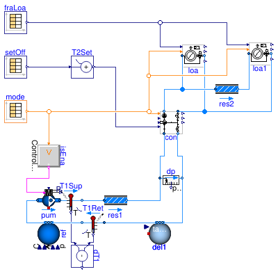
This model represents a heating system where the configuration Buildings.Fluid.HydronicConfigurations.ActiveNetworks.SingleMixing serves as the interface between a variable flow primary circuit at constant supply temperature and a constant flow secondary circuit at variable supply temperature. The primary pump is operated at constant speed so the operating point rides the pump characteristic as the three-way valve closes. The secondary supply temperature is reset with an open loop, representing for instance a reset logic based on the outdoor air temperature. Two identical terminal units are served by the secondary circuit. Each terminal unit has its own hourly load profile.
For this model to simulate properly the ratio of the Kvs coefficient
between the bypass branch and the direct branch of the control valve
(con.val.fraK) must be set to 1.
Otherwise, if con.val.fraK=0.7 cavitation occurs when
the secondary pump starts and the
control valve is fully open, as the secondary pump head
exceeds the primary pressure differential augmented by the
pressure drop across the direct branch of the control valve.
Alternatively, if the pump is sized with the pressure drop across
the direct branch of the control valve (disregarding the higher
pressure drop across the bypass) it cannot provide enough head
at low supply temperature set point when the valve is partially closed.
Note that the load loa1 is not fully met at partial load
(see plot #4 from 17 h in model time) due to the unbalanced bypass
of the terminal unit control valves.
See
Buildings.Fluid.HydronicConfigurations.ActiveNetworks.Examples.DiversionOpenLoop
for further details.
Extends from BaseClasses.PartialActivePrimary (Partial model of active primary network).
Parameters
| Type | Name | Default | Description |
|---|---|---|---|
| Control | typ | Buildings.Fluid.HydronicConf... | Load type |
| Integer | nTer | 2 | Number of terminal units |
| Real | kSizPum | 1.0 | Pump oversizing coefficient [1] |
| Pressure | p_min | 200000 | Circuit minimum pressure [Pa] |
| Temperature | TLiqEnt_nominal | if typ == Buildings.Fluid.Hy... | Liquid entering temperature at design conditions [K] |
| Temperature | TLiqLvg_nominal | TLiqEnt_nominal + (if typ ==... | Liquid leaving temperature at design conditions [K] |
| Temperature | TLiqEntChg_nominal | 60 + 273.15 | Liquid entering temperature in change-over mode [K] |
| Temperature | TLiqSup_nominal | TLiqEnt_nominal | Liquid primary supply temperature at design conditions [K] |
| Temperature | TLiqSupChg_nominal | TLiqEntChg_nominal | Liquid primary supply temperature in change-over mode [K] |
| Nominal condition | |||
| MassFlowRate | mTer_flow_nominal | 1 | Terminal unit mass flow rate at design conditions [kg/s] |
| MassFlowRate | m1_flow_nominal | m2_flow_nominal*(TLiqEnt_nom... | Mass flow rate in primary branch at design conditions [kg/s] |
| MassFlowRate | m2_flow_nominal | nTer*mTer_flow_nominal | Mass flow rate in consumer circuit at design conditions [kg/s] |
| PressureDifference | dpTer_nominal | 3E4 | Terminal unit pressure drop at design conditions [Pa] |
| PressureDifference | dpPip_nominal | 0.5E4 | Pipe section pressure drop at design conditions [Pa] |
| PressureDifference | dpPum_nominal | 10e4 | Pump head at design conditions [Pa] |
| MassFlowRate | mPum_flow_nominal | m1_flow_nominal | Primary pump mass flow rate at design conditions [kg/s] |
| Configuration | |||
| Boolean | is_bal | true | Set to true for balanced primary branch |
| Dynamics | |||
| Conservation equations | |||
| Dynamics | energyDynamics | Modelica.Fluid.Types.Dynamic... | Type of energy balance: dynamic (3 initialization options) or steady state |
Modelica definition
Buildings.Fluid.HydronicConfigurations.ActiveNetworks.Examples.ThrottleOpenLoop
Model illustrating the operation of throttle circuits with variable speed pump
Information
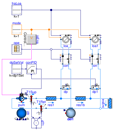
This model represents a heating system where the configuration Buildings.Fluid.HydronicConfigurations.ActiveNetworks.Throttle is used to modulate the heat flow rate transmitted to a constant load. Two identical secondary circuits are connected to a primary circuit with a variable speed pump. The pump speed is modulated to track a constant pressure differential at the boundaries of the remote circuit. The main assumptions are enumerated below.
- The model is configured in steady-state.
-
The design conditions at
time = 0are defined without considering any load diversity. -
Each consumer circuit is balanced at design conditions if the parameter
is_balis set totrue. - The pipe pressure drop between the two consumer circuits is voluntarily high to showcase typical balancing issues encountered in large distribution systems.
When simulated with the default parameter values, this example shows the following points.
-
When the consumer circuits are unbalanced (
is_bal=false), the overflow in the circuit that is the closest to the pump is about 20% (see plot #2). However, the corresponding flow shortage in the remote circuit is limited to about 2% due to equivalent flow resistance seen by the pump that is lower than design, shifting the operating point towards higher flow rates (see plot #5). The impact on the heat flow rate transferred to the load (see plot #4) is of an even lower amplitude (1%) due to the emission characteristic of the terminal unit. -
When the consumer circuits are balanced (
is_bal=true), the flow shortage in the circuit that is the closest to the pump is more significant, nearing 20% when the remote circuit has no demand (see plot #2). The impact on the heat flow rate transferred to the load (see plot #4) becomes tangible (8%) while still being not critical.
Sensitivity analysis
Those observations are confirmed by a sensitivity study to the following parameters.
- Ratio of the terminal unit pressure drop to the pump head at design conditions (refer to the schematic in the documentation of Buildings.Fluid.HydronicConfigurations.ActiveNetworks.Throttle for the nomenclature): ψ = Δp2 / Δppump varying from 0.1 to 0.4
- Ratio of the control valve authority: β = ΔpA-B / Δp1 varying from 0.1 to 0.7
-
Balanced circuit:
is_balswitched fromfalsetotrue
Valve mass flow rate
When the circuits are not balanced, Figure 1 shows that the overflow through the terminal unit closest to the pump may reach 100% of the design flow rate for low values of ψ and β. However, the concomitant flow shortage in the other terminal unit with a valve fully open is limited to about 40% and the coil capacity is reduced by less than 20% (see Figure 2). A good valve authority (higher than 0.5) does not help improving the situation.
When the circuits are balanced, the overflow is eliminated but the flow shortage is even higher (reaching 60%) and becomes critical with respect to the coil capacity that gets reduced by nearly 40%. A good valve authority (higher than 0.5) slightly helps improving the situation, which remains worse than in the case of unbalanced circuits though.
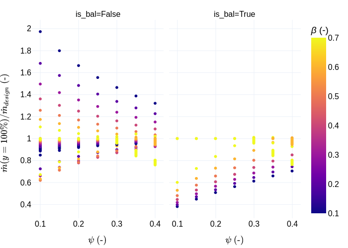
Figure 1. Valve mass flow rate (ratio to design value) at fully open conditions
as a function of
ψ for various valve authorities β (color scale),
and a circuit either balanced (right plot) or not (left plot).
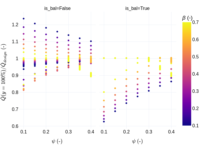
Figure 2. Heat flow rate (ratio to design value) at fully open conditions
as a function of
ψ for various valve authorities β (color scale),
and a circuit either balanced (right plot) or not (left plot).
Extends from BaseClasses.PartialActivePrimary (Partial model of active primary network).
Parameters
| Type | Name | Default | Description |
|---|---|---|---|
| Control | typ | Buildings.Fluid.HydronicConf... | Load type |
| Integer | nTer | 2 | Number of terminal units |
| Real | kSizPum | 1.0 | Pump oversizing coefficient [1] |
| Pressure | p_min | 200000 | Circuit minimum pressure [Pa] |
| Temperature | TLiqEnt_nominal | if typ == Buildings.Fluid.Hy... | Liquid entering temperature at design conditions [K] |
| Temperature | TLiqLvg_nominal | TLiqEnt_nominal + (if typ ==... | Liquid leaving temperature at design conditions [K] |
| Temperature | TLiqEntChg_nominal | 60 + 273.15 | Liquid entering temperature in change-over mode [K] |
| Temperature | TLiqSup_nominal | TLiqEnt_nominal | Liquid primary supply temperature at design conditions [K] |
| Temperature | TLiqSupChg_nominal | TLiqEntChg_nominal | Liquid primary supply temperature in change-over mode [K] |
| PressureDifference | dpValve_nominal | dpTer_nominal | Control valve pressure drop at design conditions [Pa] |
| PressureDifference | dpValve1_nominal | dpTer_nominal | Control valve pressure drop at design conditions [Pa] |
| PressureDifference | dpPip1_nominal | 3E4 | Pipe section (between two circuits) pressure drop at design conditions [Pa] |
| Nominal condition | |||
| MassFlowRate | mTer_flow_nominal | 1 | Terminal unit mass flow rate at design conditions [kg/s] |
| MassFlowRate | m1_flow_nominal | m2_flow_nominal | Mass flow rate in primary branch at design conditions [kg/s] |
| MassFlowRate | m2_flow_nominal | nTer*mTer_flow_nominal | Mass flow rate in consumer circuit at design conditions [kg/s] |
| PressureDifference | dpTer_nominal | 3E4 | Terminal unit pressure drop at design conditions [Pa] |
| PressureDifference | dpPip_nominal | 0.5E4 | Pipe section pressure drop at design conditions [Pa] |
| PressureDifference | dpPum_nominal | (dpPip_nominal + dpPip1_nomi... | Pump head at design conditions [Pa] |
| MassFlowRate | mPum_flow_nominal | m1_flow_nominal/0.9 | Primary pump mass flow rate at design conditions [kg/s] |
| Configuration | |||
| Boolean | is_bal | false | Set to true for balanced primary branch |
| ValveCharacteristic | typCha | Buildings.Fluid.HydronicConf... | Control valve characteristic |
| Controls | |||
| PressureDifference | dp1Set | dpValve1_nominal + dpTer_nom... | Pressure differential set point [Pa] |
| Dynamics | |||
| Conservation equations | |||
| Dynamics | energyDynamics | Modelica.Fluid.Types.Dynamic... | Type of energy balance: dynamic (3 initialization options) or steady state |