Buildings.Fluid.Geothermal.Borefields.BaseClasses.HeatTransfer.ThermalResponseFactors
Models for heat transfer outside boreholes
Information
This package contains functions to evaluate temperature response factors used by Buildings.Fluid.Geothermal.Borefields.BaseClasses.HeatTransfer.GroundTemperatureResponse to evaluate borehole wall temperatures.
Extends from Modelica.Icons.BasesPackage (Icon for packages containing base classes).
Package Content
| Name | Description |
|---|---|
| Cylindrical heat source solution from Carslaw and Jaeger | |
| Integrand function for cylindrical heat source evaluation | |
| Finite line source solution of Claesson and Javed | |
| Integral of the error function | |
| Integrand function for finite line source evaluation | |
| Evaluate the g-function of a bore field | |
| Infinite line source model for borehole heat exchangers | |
| Returns a SHA1 encryption of the formatted arguments for the g-function generation | |
| Geometric expansion of time steps | |
| Example models for ThermalResponseFactors |
 Buildings.Fluid.Geothermal.Borefields.BaseClasses.HeatTransfer.ThermalResponseFactors.cylindricalHeatSource
Cylindrical heat source solution from Carslaw and Jaeger
Information
This function evaluates the cylindrical heat source solution. This solution gives the relation between the constant heat transfer rate (per unit length) injected by a cylindrical heat source of infinite length and the temperature raise in the medium. The cylindrical heat source solution is defined by
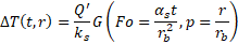
where ΔT(t,r) is the temperature raise after a time t of constant heat injection and at a distance r from the cylindrical source, Q' is the heat injection rate per unit length, ks is the soil thermal conductivity, Fo is the Fourier number, aSois is the ground thermal diffusivity, rb is the radius of the cylindrical source and G is the cylindrical heat source solution.
The cylindrical heat source solution is given by:

The integral is solved numerically, with the integrand defined in Buildings.Fluid.Geothermal.Borefields.BaseClasses.HeatTransfer.ThermalResponseFactors.cylindricalHeatSource_Integrand.
Extends from Modelica.Icons.Function (Icon for functions).
Inputs
| Type | Name | Default | Description |
|---|---|---|---|
| Time | t | Time [s] | |
| ThermalDiffusivity | aSoi | Ground thermal diffusivity [m2/s] | |
| Distance | dis | Radial distance between borehole axes [m] | |
| Radius | rBor | Radius of emitting borehole [m] |
Outputs
| Type | Name | Description |
|---|---|---|
| Real | G | Thermal response factor of borehole 1 on borehole 2 |
Modelica definition
Buildings.Fluid.Geothermal.Borefields.BaseClasses.HeatTransfer.ThermalResponseFactors.cylindricalHeatSource_Integrand
Integrand function for cylindrical heat source evaluation
Information
Integrand of the cylindrical heat source solution for use in Buildings.Fluid.Geothermal.Borefields.BaseClasses.HeatTransfer.ThermalResponseFactors.cylindricalHeatSource.
Extends from Modelica.Icons.Function (Icon for functions).
Inputs
| Type | Name | Default | Description |
|---|---|---|---|
| Real | u | Normalized integration variable | |
| Real | Fo | Fourier number | |
| Real | p | Ratio of distance over radius |
Outputs
| Type | Name | Description |
|---|---|---|
| Real | y | Value of integrand |
Modelica definition
Buildings.Fluid.Geothermal.Borefields.BaseClasses.HeatTransfer.ThermalResponseFactors.finiteLineSource
Finite line source solution of Claesson and Javed
Information
This function evaluates the finite line source solution. This solution gives the relation between the constant heat transfer rate (per unit length) injected by a line source of finite length H1 buried at a distance D1 from a constant temperature surface (T=0) and the average temperature raise over a line of finite length H2 buried at a distance D2 from the constant temperature surface. The finite line source solution is defined by:
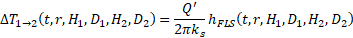
where ΔT1-2(t,r,H1,D1,H2,D2) is the temperature raise after a time t of constant heat injection and at a distance r from the line heat source, Q' is the heat injection rate per unit length, ks is the soil thermal conductivity and hFLS is the finite line source solution.
The finite line source solution is given by:
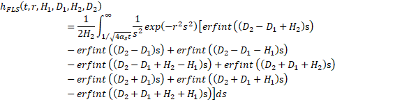
where αs is the ground thermal diffusivity and erfint is the integral of the error function, defined in Buildings.Fluid.Geothermal.Borefields.BaseClasses.HeatTransfer.ThermalResponseFactors.finiteLineSource_erfint. The integral is solved numerically, with the integrand defined in Buildings.Fluid.Geothermal.Borefields.BaseClasses.HeatTransfer.ThermalResponseFactors.finiteLineSource_Integrand.
Extends from Modelica.Icons.Function (Icon for functions).
Inputs
| Type | Name | Default | Description |
|---|---|---|---|
| Time | t | Time [s] | |
| ThermalDiffusivity | aSoi | Ground thermal diffusivity [m2/s] | |
| Distance | dis | Radial distance between borehole axes [m] | |
| Height | len1 | Length of emitting borehole [m] | |
| Height | burDep1 | Buried depth of emitting borehole [m] | |
| Height | len2 | Length of receiving borehole [m] | |
| Height | burDep2 | Buried depth of receiving borehole [m] | |
| Boolean | includeRealSource | true | True if contribution of real source is included |
| Boolean | includeMirrorSource | true | True if contribution of mirror source is included |
Outputs
| Type | Name | Description |
|---|---|---|
| Real | h_21 | Thermal response factor of borehole 1 on borehole 2 |
Modelica definition
Buildings.Fluid.Geothermal.Borefields.BaseClasses.HeatTransfer.ThermalResponseFactors.finiteLineSource_Erfint
Integral of the error function
Information
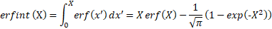
This function evaluates the integral of the error function, given by:
Extends from Modelica.Math.Nonlinear.Interfaces.partialScalarFunction (Interface for a function with one input and one output Real signal).
Inputs
| Type | Name | Default | Description |
|---|---|---|---|
| Real | u | Independent variable |
Outputs
| Type | Name | Description |
|---|---|---|
| Real | y | Dependent variable y=f(u) |
Modelica definition
Buildings.Fluid.Geothermal.Borefields.BaseClasses.HeatTransfer.ThermalResponseFactors.finiteLineSource_Integrand
Integrand function for finite line source evaluation
Information
Integrand of the cylindrical heat source solution for use in Buildings.Fluid.Geothermal.Borefields.BaseClasses.HeatTransfer.ThermalResponseFactors.finiteLineSource.
Extends from Modelica.Icons.Function (Icon for functions).
Inputs
| Type | Name | Default | Description |
|---|---|---|---|
| Real | u | Integration variable [1/m] | |
| Distance | dis | Radial distance between borehole axes [m] | |
| Height | len1 | Length of emitting borehole [m] | |
| Height | burDep1 | Buried depth of emitting borehole [m] | |
| Height | len2 | Length of receiving borehole [m] | |
| Height | burDep2 | Buried depth of receiving borehole [m] | |
| Boolean | includeRealSource | true | true if contribution of real source is included |
| Boolean | includeMirrorSource | true | true if contribution of mirror source is included |
Outputs
| Type | Name | Description |
|---|---|---|
| Real | y | Value of integrand [m] |
Modelica definition
Buildings.Fluid.Geothermal.Borefields.BaseClasses.HeatTransfer.ThermalResponseFactors.gFunction
Evaluate the g-function of a bore field
Information
This function implements the g-function evaluation method introduced by Cimmino and Bernier (see: Cimmino and Bernier (2014), and Cimmino (2018)) based on the g-function function concept first introduced by Eskilson (1987). The g-function gives the relation between the variation of the borehole wall temperature at a time t and the heat extraction and injection rates at all times preceding time t as
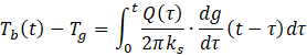
where Tb is the borehole wall temperature, Tg is the undisturbed ground temperature, Q is the heat injection rate into the ground through the borehole wall per unit borehole length, ks is the soil thermal conductivity and g is the g-function.
The g-function is constructed from the combination of the combination of
the finite line source (FLS) solution (see
Buildings.Fluid.Geothermal.Borefields.BaseClasses.HeatTransfer.ThermalResponseFactors.finiteLineSource),
the cylindrical heat source (CHS) solution (see
Buildings.Fluid.Geothermal.Borefields.BaseClasses.HeatTransfer.ThermalResponseFactors.cylindricalHeatSource),
and the infinite line source (ILS) solution (see
Buildings.Fluid.Geothermal.Borefields.BaseClasses.HeatTransfer.ThermalResponseFactors.infiniteLineSource).
To obtain the g-function of a bore field, each borehole is divided into a
series of nSeg segments of equal length, each modeled as a line
source of finite length. The finite line source solution is superimposed in
space to obtain a system of equations that gives the relation between the heat
injection rate at each of the segments and the borehole wall temperature at each
of the segments. The system is solved to obtain the uniform borehole wall
temperature required at any time to maintain a constant total heat injection
rate (Qtot = 2πksHtot) into the bore
field. The uniform borehole wall temperature is then equal to the finite line
source based g-function.
Since this g-function is based on line sources of heat, rather than cylinders, the g-function is corrected to consider the cylindrical geometry. The correction factor is then the difference between the cylindrical heat source solution and the infinite line source solution, as proposed by Li et al. (2014) as
g(t) = gFLS + (gCHS - gILS)
Implementation
The calculation of the g-function is separated into two regions: the
short-time region and the long-time region. In the short-time region,
corresponding to times t < 1 hour, heat interaction between boreholes
and axial variations of heat injection rate are not considered. The
g-function is calculated using only one borehole and one segment. In the
long-time region, corresponding to times t > 1 hour, all boreholes
are represented as series of nSeg line segments and the
g-function is evaluated as described above.
References
Cimmino, M. and Bernier, M. 2014. A semi-analytical method to generate g-functions for geothermal bore fields. International Journal of Heat and Mass Transfer 70: 641-650.
Cimmino, M. 2018. Fast calculation of the g-functions of geothermal borehole fields using similarities in the evaluation of the finite line source solution. Journal of Building Performance Simulation. DOI: 10.1080/19401493.2017.1423390.
Eskilson, P. 1987. Thermal analysis of heat extraction boreholes. Ph.D. Thesis. Department of Mathematical Physics. University of Lund. Sweden.
Li, M., Li, P., Chan, V. and Lai, A.C.K. 2014. Full-scale temperature response function (G-function) for heat transfer by borehole heat exchangers (GHEs) from sub-hour to decades. Applied Energy 136: 197-205.
Extends from Modelica.Icons.Function (Icon for functions).
Inputs
| Type | Name | Default | Description |
|---|---|---|---|
| Integer | nBor | Number of boreholes | |
| Position | cooBor[nBor, 2] | Coordinates of boreholes [m] | |
| Height | hBor | Borehole length [m] | |
| Height | dBor | Borehole buried depth [m] | |
| Radius | rBor | Borehole radius [m] | |
| ThermalDiffusivity | aSoi | Ground thermal diffusivity used in g-function evaluation [m2/s] | |
| Integer | nSeg | Number of line source segments per borehole | |
| Integer | nTimSho | Number of time steps in short time region | |
| Integer | nTimLon | Number of time steps in long time region | |
| Real | ttsMax | Maximum adimensional time for gfunc calculation | |
| Real | relTol | 0.02 | Relative tolerance on distance between boreholes |
Outputs
| Type | Name | Description |
|---|---|---|
| Time | tGFun[nTimSho + nTimLon] | Time of g-function evaluation [s] |
| Real | g[nTimSho + nTimLon] | g-function |
Modelica definition
Buildings.Fluid.Geothermal.Borefields.BaseClasses.HeatTransfer.ThermalResponseFactors.infiniteLineSource
Infinite line source model for borehole heat exchangers
Information
This function evaluates the infinite line source solution. This solution gives the relation between the constant heat transfer rate (per unit length) injected by a line heat source of infinite length and the temperature raise in the medium. The infinite line source solution is defined by
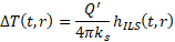
where ΔT(t,r) is the temperature raise after a time t of constant heat injection and at a distance r from the line source, Q' is the heat injection rate per unit length, ks is the soil thermal conductivity and hILS is the infinite line source solution.
The infinite line source solution is given by the exponential integral
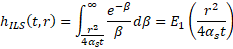
where αs is the ground thermal diffusivity. The exponential integral is implemented in Buildings.Utilities.Math.Functions.exponentialIntegralE1.
Extends from Modelica.Icons.Function (Icon for functions).
Inputs
| Type | Name | Default | Description |
|---|---|---|---|
| Real | t | Time | |
| Real | aSoi | Ground thermal diffusivity | |
| Real | dis | Radial distance between borehole axes |
Outputs
| Type | Name | Description |
|---|---|---|
| Real | h_ils | Thermal response factor of borehole 1 on borehole 2 |
Modelica definition
Buildings.Fluid.Geothermal.Borefields.BaseClasses.HeatTransfer.ThermalResponseFactors.shaGFunction
Returns a SHA1 encryption of the formatted arguments for the g-function generation
Information
This function returns the SHA1 encryption of its arguments.
Implementation
Each argument is formatted in exponential notation
with four significant digits, for example 1.234e+001, with no spaces or
other separating characters between each argument value.
To prevent too long strings that can cause buffer overflows,
the sha encoding of each argument is computed and added to the next string that
is parsed.
The SHA1 encryption is computed using Buildings.Utilities.Cryptographics.sha.
Extends from Modelica.Icons.Function (Icon for functions).
Inputs
| Type | Name | Default | Description |
|---|---|---|---|
| Integer | nBor | Number of boreholes | |
| Position | cooBor[nBor, 2] | Coordinates of boreholes [m] | |
| Height | hBor | Borehole length [m] | |
| Height | dBor | Borehole buried depth [m] | |
| Radius | rBor | Borehole radius [m] | |
| ThermalDiffusivity | aSoi | Ground thermal diffusivity used in g-function evaluation [m2/s] | |
| Integer | nSeg | Number of line source segments per borehole | |
| Integer | nTimSho | Number of time steps in short time region | |
| Integer | nTimLon | Number of time steps in long time region | |
| Real | ttsMax | Maximum adimensional time for gfunc calculation |
Outputs
| Type | Name | Description |
|---|---|---|
| String | sha | SHA1 encryption of the g-function arguments |
Modelica definition
Buildings.Fluid.Geothermal.Borefields.BaseClasses.HeatTransfer.ThermalResponseFactors.timeGeometric
Geometric expansion of time steps
Information
This function attemps to build a vector of length nTim with a geometric
expansion of the time variable between dt and t_max.
If t_max > nTim*dt, then a geometrically expanding vector is built as
t = [dt, dt*(1-r2)/(1-r), ... , dt*(1-rn)/(1-r), ... , tmax],
where r is the geometric expansion factor.
If t_max < nTim*dt, then a linearly expanding vector is built as
t = [dt, 2*dt, ... , n*dt, ... , nTim*dt]
Extends from Modelica.Icons.Function (Icon for functions).
Inputs
| Type | Name | Default | Description |
|---|---|---|---|
| Duration | dt | Minimum time step [s] | |
| Time | t_max | Maximum value of time [s] | |
| Integer | nTim | Number of time values |
Outputs
| Type | Name | Description |
|---|---|---|
| Real | t[nTim] | Time vector |