Buildings.Fluid.Geothermal.Borefields.BaseClasses.HeatTransfer

Package with ground heat transfer models

Information

This package contains models and functions to solve ground heat transfer around ground heat exchangers. For more information on the model implementation, see the documentation of Buildings.Fluid.Geothermal.Borefields.BaseClasses.HeatTransfer.GroundTemperatureResponse.

Extends from Modelica.Icons.VariantsPackage (Icon for package containing variants).

Package Content

Name Description
Buildings.Fluid.Geothermal.Borefields.BaseClasses.HeatTransfer.Cylindrical Cylindrical Heat conduction in a cylinder using the radial discretization as advised by Eskilson
Buildings.Fluid.Geothermal.Borefields.BaseClasses.HeatTransfer.GroundTemperatureResponse GroundTemperatureResponse Model calculating discrete load aggregation
Buildings.Fluid.Geothermal.Borefields.BaseClasses.HeatTransfer.LoadAggregation LoadAggregation Package with functions for load aggregation
Buildings.Fluid.Geothermal.Borefields.BaseClasses.HeatTransfer.ThermalResponseFactors ThermalResponseFactors Models for heat transfer outside boreholes
Buildings.Fluid.Geothermal.Borefields.BaseClasses.HeatTransfer.Validation Validation Validation models for GroundHeatTransfer

Buildings.Fluid.Geothermal.Borefields.BaseClasses.HeatTransfer.Cylindrical Buildings.Fluid.Geothermal.Borefields.BaseClasses.HeatTransfer.Cylindrical

Heat conduction in a cylinder using the radial discretization as advised by Eskilson

Buildings.Fluid.Geothermal.Borefields.BaseClasses.HeatTransfer.Cylindrical

Information

Model for radial heat transfer in a hollow cylinder.

If the heat capacity of the material is non-zero, then this model computes transient heat conduction, i.e., it computes a numerical approximation to the solution of the heat equation

ρ c ( ∂ T(r,t) ⁄ ∂t ) = k ( ∂² T(r,t) ⁄ ∂r² + 1 ⁄ r   ∂ T(r,t) ⁄ ∂r ),

where ρ is the mass density, c is the specific heat capacity per unit mass, T is the temperature at location r and time t and k is the heat conductivity. At the locations r=ra and r=rb, the temperature and heat flow rate are equal to the temperature and heat flow rate of the heat ports.

If the heat capacity of the material is set to zero, then steady-state heat flow is computed using

Q = 2 π k (Ta-Tb)⁄ ln(ra ⁄ rb),

where ra is the internal radius, rb is the external radius, Ta is the temperature at port a and Tb is the temperature at port b.

Implementation

To spatially discretize the heat equation, the construction is divided into compartments with nSta ≥ 1 state variables. The state variables are connected to each other through thermal conductors. There is also a thermal conductor between the surfaces and the outermost state variables. Thus, to obtain the surface temperature, use port_a.T (or port_b.T) and not the variable T[1].

Parameters

TypeNameDefaultDescription
TemplatesoiDat  
Heighth Height of the cylinder [m]
Radiusr_a Internal radius [m]
Radiusr_b External radius [m]
IntegernSta10Number of state variables
RealgridFac2Grid factor for spacing
Radiusr[nSta + 1] Radius to the boundary of the i-th domain [m]
Initialization
TemperatureTInt_start Initial temperature at port_a, used if steadyStateInitial = false [K]
TemperatureTExt_start Initial temperature at port_b, used if steadyStateInitial = false [K]
BooleansteadyStateInitialfalsetrue initializes dT(0)/dt=0, false initializes T(0) at fixed temperature using T_a_start and T_b_start

Connectors

TypeNameDescription
HeatPort_aport_aHeat port at surface a
HeatPort_bport_bHeat port at surface b

Modelica definition

model Cylindrical "Heat conduction in a cylinder using the radial discretization as advised by Eskilson" parameter Buildings.Fluid.Geothermal.Borefields.Data.Soil.Template soiDat; parameter Modelica.Units.SI.Height h "Height of the cylinder"; parameter Modelica.Units.SI.Radius r_a "Internal radius"; parameter Modelica.Units.SI.Radius r_b "External radius"; parameter Integer nSta(min=1) = 10 "Number of state variables"; parameter Modelica.Units.SI.Temperature TInt_start "Initial temperature at port_a, used if steadyStateInitial = false"; parameter Modelica.Units.SI.Temperature TExt_start "Initial temperature at port_b, used if steadyStateInitial = false"; parameter Boolean steadyStateInitial=false "true initializes dT(0)/dt=0, false initializes T(0) at fixed temperature using T_a_start and T_b_start"; parameter Real gridFac(min=1) = 2 "Grid factor for spacing"; parameter Modelica.Units.SI.Radius r[nSta + 1](each fixed=false) "Radius to the boundary of the i-th domain"; Modelica.Thermal.HeatTransfer.Interfaces.HeatPort_a port_a(T(start=TInt_start)) "Heat port at surface a"; Modelica.Thermal.HeatTransfer.Interfaces.HeatPort_b port_b(T(start=TExt_start)) "Heat port at surface b"; Modelica.Units.SI.Temperature T[nSta](start={TInt_start + (TExt_start - TInt_start)/Modelica.Math.log(r_b/r_a)*Modelica.Math.log((r_a + (r_b - r_a)/(nSta)*(i - 0.5))/r_a) for i in 1:nSta}) "Temperature of the states"; Modelica.Units.SI.TemperatureDifference dT "port_a.T - port_b.T"; Modelica.Units.SI.HeatFlowRate Q_flow[nSta + 1] "Heat flow rate from state i to i+1"; protected parameter Modelica.Units.SI.Radius rC[nSta](each fixed=false) "Radius to the center of the i-th domain"; final parameter Modelica.Units.SI.SpecificHeatCapacity c=soiDat.cSoi "Specific heat capacity"; final parameter Modelica.Units.SI.ThermalConductivity k=soiDat.kSoi "Thermal conductivity of the material"; final parameter Modelica.Units.SI.Density d=soiDat.dSoi "Density of the material"; parameter Modelica.Units.SI.ThermalConductance G[nSta + 1](each fixed=false) "Heat conductance between the temperature nodes"; parameter Modelica.Units.SI.HeatCapacity C[nSta](each fixed=false) "Heat capacity of each state"; parameter Real gridFac_sum(fixed=false); parameter Real gridFac_sum_old(fixed=false); initial algorithm for i in 0:nSta - 3 - 1 loop if i == 0 then gridFac_sum := gridFac^i; gridFac_sum_old := gridFac_sum; else gridFac_sum := gridFac_sum_old + gridFac^i; gridFac_sum_old := gridFac_sum; end if; end for; initial equation assert(r_a < r_b, "Error: Model requires r_a < r_b."); assert(0 < r_a, "Error: Model requires 0 < r_a."); // ****************** Comments *********************: // The layer is divided into nSta segments. The radius of each segment increase exponentially with base 'griFac': // r_b - r_a = sum( a * griFac^k - a , k=2..nSta) => from this we find a = (r_b - r_a)/(griFac^(n+1) - griFac) // Using this a, we can now find the r[i]: // r[1] := r_a // r[i] = r[i-1] + a * griFac^i = r[i-1] + griFac^i * (r_b - r_a) / (griFac^(n+1) - griFac) // // This can also be writing as: // r[i]= r[i-1] + ( r_b - r_a) * (1-griFac)/(1-griFac^(nSta)) * griFac^(i-2); r[1] = r_a; r[2] = r_a + sqrt(k/c/d*60) "eskilson minimum length"; r[3] = r_a + 2*sqrt(k/c/d*60); r[4] = r_a + 3*sqrt(k/c/d*60); for i in 5:nSta + 1 loop r[i] = r[i - 1] + (r_b - r[4])/gridFac_sum*gridFac^(i - 5); end for; assert(abs(r[nSta + 1] - r_b) < 1E-3, "Error: Wrong computation of radius. r[nSta+1]=" + String(r[nSta + 1])); // Radii at middle of resistance for i in 1:nSta loop rC[i] = (r[i] + r[i + 1])/2; end for; // Conductance between nodes (which are in the center of the domain) G[1] = 2*Modelica.Constants.pi*k*h/Modelica.Math.log(rC[1]/r_a); G[nSta + 1] = 2*Modelica.Constants.pi*k*h/Modelica.Math.log(r_b/rC[nSta]); for i in 2:nSta loop G[i] = 2*Modelica.Constants.pi*k*h/Modelica.Math.log(rC[i]/rC[i - 1]); end for; // Heat capacity of each segment for i in 1:nSta loop C[i] = (d*Modelica.Constants.pi*c*h*((r[i + 1])^2 - (r[i])^2)); end for; // The initialization is only done for materials that store energy. if not soiDat.steadyState then if steadyStateInitial then der(T) = zeros(nSta); else for i in 1:nSta loop T[i] = TInt_start + (TExt_start - TInt_start)/Modelica.Math.log(r_b/r_a) *Modelica.Math.log(rC[i]/r_a); end for; end if; end if; equation dT = port_a.T - port_b.T; port_a.Q_flow = +Q_flow[1]; port_b.Q_flow = -Q_flow[nSta + 1]; Q_flow[1] = G[1]*(port_a.T - T[1]); Q_flow[nSta + 1] = G[nSta + 1]*(T[nSta] - port_b.T); for i in 2:nSta loop Q_flow[i] = G[i]*(T[i - 1] - T[i]); // Q_flow[i] represents the heat flowing between two nodes end for; if soiDat.steadyState then for i in 2:nSta + 1 loop Q_flow[i] = Q_flow[1]; end for; else for i in 1:nSta loop der(T[i]) = (Q_flow[i] - Q_flow[i + 1])/C[i]; end for; end if; end Cylindrical;

Buildings.Fluid.Geothermal.Borefields.BaseClasses.HeatTransfer.GroundTemperatureResponse Buildings.Fluid.Geothermal.Borefields.BaseClasses.HeatTransfer.GroundTemperatureResponse

Model calculating discrete load aggregation

Buildings.Fluid.Geothermal.Borefields.BaseClasses.HeatTransfer.GroundTemperatureResponse

Information

This model calculates the ground temperature response to obtain the temperature at the borehole wall in a geothermal system where heat is being injected into or extracted from the ground.

A load-aggregation scheme based on that developed by Claesson and Javed (2012) is used to calculate the borehole wall temperature response with the temporal superposition of ground thermal loads. In its base form, the load-aggregation scheme uses fixed-length aggregation cells to agglomerate thermal load history together, with more distant cells (denoted with a higher cell and vector index) representing more distant thermal history. The more distant the thermal load, the less impactful it is on the borehole wall temperature change at the current time step. Each cell has an aggregation time associated to it denoted by nu, which corresponds to the simulation time (since the beginning of heat injection or extraction) at which the cell will begin shifting its thermal load to more distant cells. To determine nu, cells have a temporal size rcel (rcel in this model) which follows the exponential growth

image

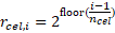
where nCel is the number of consecutive cells which can have the same size. Decreasing rcel will generally decrease calculation times, at the cost of precision in the temporal superposition. rcel is expressed in multiples of the aggregation time resolution (via the parameter tLoaAgg). Then, nu may be expressed as the sum of all rcel values (multiplied by the aggregation time resolution) up to and including that cell in question.

To determine the weighting factors, the borefield's temperature step response at the borefield wall is determined as

image

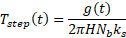
where g(·) is the borefield's thermal response factor known as the g-function, H is the total length of all boreholes and ks is the thermal conductivity of the soil. The weighting factors kappa (κ in the equation below) for a given cell i are then expressed as follows.

image

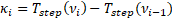
where ν refers to the vector nu in this model and Tstep0)=0.

At every aggregation time step, a time event is generated to perform the load aggregation steps. First, the thermal load is shifted. When shifting between cells of different size, total energy is conserved. This operation is illustred in the figure below by Cimmino (2014).

image

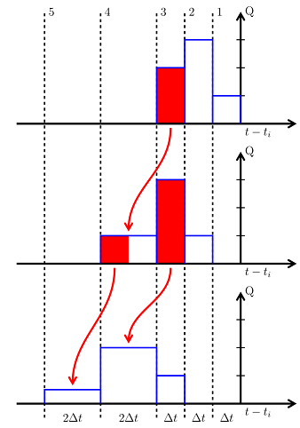
After the cell-shifting operation is performed, the first aggregation cell has its value set to the average thermal load since the last aggregation step. Temporal superposition is then applied by means of a scalar product between the aggregated thermal loads QAgg_flow and the weighting factors κ.

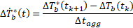
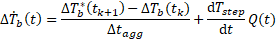
Due to Modelica's variable time steps, the load aggregation scheme is modified by separating the thermal response between the current aggregation time step and everything preceding it. This is done according to

image
image

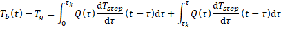
where Tb is the borehole wall temperature, Tg is the undisturbed ground temperature, Q is the ground thermal load per borehole length and h = g/(2 π ks) is a temperature response factor based on the g-function. tk is the last discrete aggregation time step, meaning that the current time t satisfies tk≤t≤tk+1. Δtagg(=tk+1-tk) is the parameter tLoaAgg in the present model.

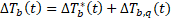
Thus, ΔTb*(t) is the borehole wall temperature change due to the thermal history prior to the current aggregation step. At every aggregation time step, load aggregation and temporal superposition are used to calculate its discrete value. Assuming no heat injection or extraction until tk+1, this term is assumed to have a linear time derivative, which is given by the difference between ΔTb*(tk+1) (the temperature change from load history at the next discrete aggregation time step, which is constant over the duration of the ongoing aggregation time step) and the total temperature change at the last aggregation time step, ΔTb(t).

image

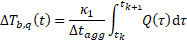
The second term ΔTb,q(t) concerns the ongoing aggregation time step. To obtain the time derivative of this term, the thermal response factor h is assumed to vary linearly over the course of an aggregation time step. Therefore, because the ongoing aggregation time step always concerns the first aggregation cell, its derivative (denoted 
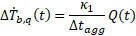
by the parameter dTStepdt in this model) can be calculated as kappa[1], the first value in the kappa vector, divided by the aggregation time step Δt. 
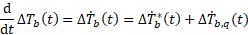
The derivative of the temperature change at the borehole wall is then expressed as the multiplication of dTStepdt (which only needs to be calculated once at the start of the simulation) and the heat flow Q at the borehole wall.

image

image

With the two terms in the expression of ΔTb(t) expressed as time derivatives, ΔTb(t) can itself also be expressed as its time derivative and implemented as such directly in the Modelica equations block with the der() operator.

image
image

This load aggregation scheme is validated in Buildings.Fluid.Geothermal.Borefields.BaseClasses.HeatTransfer.Validation.Analytic_20Years.

References

Cimmino, M. 2014. Développement et validation expérimentale de facteurs de réponse thermique pour champs de puits géothermiques, Ph.D. Thesis, École Polytechnique de Montréal.

Claesson, J. and Javed, S. 2012. A load-aggregation method to calculate extraction temperatures of borehole heat exchangers. ASHRAE Transactions 118(1): 530-539.

Parameters

TypeNameDefaultDescription
TimetLoaAgg3600Time resolution of load aggregation [s]
IntegernCel5Number of cells per aggregation level
BooleanforceGFunCalcfalseSet to true to force the thermal response to be calculated at the start instead of checking whether it has been pre-computed
TemplateborFieDat Record containing all the parameters of the borefield model

Connectors

TypeNameDescription
output RealOutputdelTBorTemperature difference current borehole wall temperature minus initial borehole wall temperature [K]
input RealInputQBor_flowHeat flow from all boreholes combined (positive if heat from fluid into soil) [W]

Modelica definition

model GroundTemperatureResponse "Model calculating discrete load aggregation" parameter Modelica.Units.SI.Time tLoaAgg(final min=Modelica.Constants.eps) = 3600 "Time resolution of load aggregation"; parameter Integer nCel(min=1)=5 "Number of cells per aggregation level"; parameter Boolean forceGFunCalc = false "Set to true to force the thermal response to be calculated at the start instead of checking whether it has been pre-computed"; parameter Buildings.Fluid.Geothermal.Borefields.Data.Borefield.Template borFieDat "Record containing all the parameters of the borefield model"; Modelica.Blocks.Interfaces.RealOutput delTBor(unit="K") "Temperature difference current borehole wall temperature minus initial borehole wall temperature"; Modelica.Blocks.Interfaces.RealInput QBor_flow(unit="W") "Heat flow from all boreholes combined (positive if heat from fluid into soil)"; protected constant Integer nSegMax = 1500 "Max total number of segments in g-function calculation"; final parameter Integer nSeg = integer(if 12*borFieDat.conDat.nBor<nSegMax then 12 else floor(nSegMax/borFieDat.conDat.nBor)) "Number of segments per borehole for g-function calculation"; constant Integer nTimSho = 26 "Number of time steps in short time region"; constant Integer nTimLon = 50 "Number of time steps in long time region"; constant Real ttsMax = exp(5) "Maximum non-dimensional time for g-function calculation"; constant Integer nTimTot = nTimSho+nTimLon "Total length of g-function vector"; constant Real lvlBas = 2 "Base for exponential cell growth between levels"; parameter String SHAgfun= Buildings.Fluid.Geothermal.Borefields.BaseClasses.HeatTransfer.ThermalResponseFactors.shaGFunction( nBor=borFieDat.conDat.nBor, cooBor=borFieDat.conDat.cooBor, hBor=borFieDat.conDat.hBor, dBor=borFieDat.conDat.dBor, rBor=borFieDat.conDat.rBor, aSoi=borFieDat.soiDat.aSoi, nSeg=nSeg, nTimSho=nTimSho, nTimLon=nTimLon, ttsMax=ttsMax) "String with encrypted g-function arguments"; parameter Modelica.Units.SI.Time timFin=(borFieDat.conDat.hBor^2/(9*borFieDat.soiDat.aSoi)) *ttsMax "Final time for g-function calculation"; parameter Integer i(min=1)= Buildings.Fluid.Geothermal.Borefields.BaseClasses.HeatTransfer.LoadAggregation.countAggregationCells( lvlBas=lvlBas, nCel=nCel, timFin=timFin, tLoaAgg=tLoaAgg) "Number of aggregation cells"; final parameter Real[nTimTot,2] timSer(each fixed=false) "g-function input from matrix, with the second column as temperature Tstep"; final parameter Modelica.Units.SI.Time t_start(fixed=false) "Simulation start time"; final parameter Modelica.Units.SI.Time[i] nu(each fixed=false) "Time vector for load aggregation"; final parameter Real[i] kappa(each fixed=false) "Weight factor for each aggregation cell"; final parameter Real[i] rCel(each fixed=false) "Cell widths"; discrete Modelica.Units.SI.HeatFlowRate[i] QAgg_flow "Vector of aggregated loads"; discrete Modelica.Units.SI.HeatFlowRate[i] QAggShi_flow "Shifted vector of aggregated loads"; discrete Integer curCel "Current occupied cell"; discrete Modelica.Units.SI.TemperatureDifference delTBor0 "Previous time step's temperature difference current borehole wall temperature minus initial borehole temperature"; discrete Real derDelTBor0(unit="K/s") "Derivative of wall temperature change from previous time steps"; final parameter Real dTStepdt(fixed=false) "Time derivative of g/(2*pi*H*Nb*ks) within most recent cell"; Modelica.Units.SI.Heat U "Accumulated heat flow from all boreholes"; discrete Modelica.Units.SI.Heat U_old "Accumulated heat flow from all boreholes at last aggregation step"; initial equation QAgg_flow = zeros(i); curCel = 1; delTBor = 0; QAggShi_flow = QAgg_flow; delTBor0 = 0; U = 0; U_old = 0; derDelTBor0 = 0; (nu,rCel) = Buildings.Fluid.Geothermal.Borefields.BaseClasses.HeatTransfer.LoadAggregation.aggregationCellTimes( i=i, lvlBas=lvlBas, nCel=nCel, tLoaAgg=tLoaAgg, timFin=timFin); t_start = time; kappa = Buildings.Fluid.Geothermal.Borefields.BaseClasses.HeatTransfer.LoadAggregation.aggregationWeightingFactors( i=i, nTimTot=nTimTot, TStep=timSer, nu=nu); dTStepdt = kappa[1]/tLoaAgg; timSer = Buildings.Fluid.Geothermal.Borefields.BaseClasses.HeatTransfer.LoadAggregation.temperatureResponseMatrix( nBor=borFieDat.conDat.nBor, cooBor=borFieDat.conDat.cooBor, hBor=borFieDat.conDat.hBor, dBor=borFieDat.conDat.dBor, rBor=borFieDat.conDat.rBor, aSoi=borFieDat.soiDat.aSoi, kSoi=borFieDat.soiDat.kSoi, nSeg=nSeg, nTimSho=nTimSho, nTimLon=nTimLon, nTimTot=nTimTot, ttsMax=ttsMax, sha=SHAgfun, forceGFunCalc=forceGFunCalc); equation der(delTBor) = dTStepdt*QBor_flow + derDelTBor0; der(U) = QBor_flow; when sample(t_start, tLoaAgg) then // Assign average load since last aggregation step to the first cell of the // aggregation vector U_old = U; // Store (U - pre(U_old))/tLoaAgg in QAgg_flow[1], and pre(QAggShi_flow) in the other elements QAgg_flow = cat(1, {(U - pre(U_old))/tLoaAgg}, pre(QAggShi_flow[2:end])); // Shift loads in aggregation cells (curCel,QAggShi_flow) = Buildings.Fluid.Geothermal.Borefields.BaseClasses.HeatTransfer.LoadAggregation.shiftAggregationCells( i=i, QAgg_flow=QAgg_flow, rCel=rCel, nu=nu, curTim=(time - t_start)); // Determine the temperature change at the next aggregation step (assuming // no loads until then) delTBor0 = Buildings.Fluid.Geothermal.Borefields.BaseClasses.HeatTransfer.LoadAggregation.temporalSuperposition( i=i, QAgg_flow=QAggShi_flow, kappa=kappa, curCel=curCel); derDelTBor0 = (delTBor0-delTBor)/tLoaAgg; end when; end GroundTemperatureResponse;