Buildings.Fluid.Chillers

Home > Modelica

Buildings.Fluid.Chillers

Package with chiller models

Information

This package contains components models for chillers. The model Buildings.Fluid.Chillers.Carnot computes the coefficient of performance based on a change in the Carnot effectiveness. The models Buildings.Fluid.Chillers.ElectricReformulatedEIR and Buildings.Fluid.Chillers.ElectricEIR use performance curves from the package Buildings.Fluid.Chillers.Data to compute the chiller performance.

Extends from Modelica.Icons.VariantsPackage (Icon for package containing variants).

Package Content

Name Description

Carnot Chiller with performance curve adjusted based on Carnot efficiency

ElectricReformulatedEIR Electric chiller based on the DOE-2.1 model, but with performance as a function of condenser leaving instead of entering temperature

ElectricEIR Electric chiller based on the DOE-2.1 model

Examples Collection of models that illustrate model use and test models

Data Performance data for electric chillers

BaseClasses Package with base classes for Buildings.Fluid.Chillers

Name	Description
Carnot	Chiller with performance curve adjusted based on Carnot efficiency
ElectricReformulatedEIR	Electric chiller based on the DOE-2.1 model, but with performance as a function of condenser leaving instead of entering temperature
ElectricEIR	Electric chiller based on the DOE-2.1 model
Examples	Collection of models that illustrate model use and test models
Data	Performance data for electric chillers
BaseClasses	Package with base classes for Buildings.Fluid.Chillers

Buildings.Fluid.Chillers.Carnot

Chiller with performance curve adjusted based on Carnot efficiency

Buildings.Fluid.Chillers.Carnot

Information

This is model of a chiller whose coefficient of performance (COP) changes with temperatures in the same way as the Carnot efficiency changes. The COP at the nominal conditions can be specified by a parameter, or it can be computed by the model based on the Carnot effectiveness, in which case

COP₀ = η_car COP_car = η_car T_eva ⁄ (T_con-T_eva),

where T_eva is the evaporator temperature and T_con is the condenser temperature. On the Advanced tab, a user can specify the temperature that will be used as the evaporator (or condenser) temperature. The options are the temperature of the fluid volume, of port_a, of port_b, or the average temperature of port_a and port_b.

The chiller COP is computed as the product

COP = η_car COP_car η_PL,

where η_car is the Carnot effectiveness, COP_car is the Carnot efficiency and η_PL is a polynomial in the control signal y that can be used to take into account a change in COP at part load conditions.

On the Dynamics tag, the model can be parametrized to compute a transient or steady-state response. The transient response of the model is computed using a first order differential equation for the evaporator and condenser fluid volumes. The chiller outlet temperatures are equal to the temperatures of these lumped volumes.

Extends from Interfaces.FourPortHeatMassExchanger (Model transporting two fluid streams between four ports with storing mass or energy).

Parameters

Type Name Default Description

replaceable package Medium1 PartialMedium Medium 1 in the component

replaceable package Medium2 PartialMedium Medium 2 in the component

Nominal condition

MassFlowRate m1_flow_nominal Nominal mass flow rate [kg/s]

MassFlowRate m2_flow_nominal Nominal mass flow rate [kg/s]

Pressure dp1_nominal Pressure [Pa]

Pressure dp2_nominal Pressure [Pa]

Power P_nominal Nominal compressor power (at y=1) [W]

TemperatureDifference dTEva_nominal 10 Temperature difference evaporator inlet-outlet [K]

TemperatureDifference dTCon_nominal 10 Temperature difference condenser outlet-inlet [K]

Initialization

MassFlowRate m1_flow.start 0 Mass flow rate from port_a1 to port_b1 (m1_flow > 0 is design flow direction) [kg/s]

Pressure dp1.start 0 Pressure difference between port_a1 and port_b1 [Pa]

MassFlowRate m2_flow.start 0 Mass flow rate from port_a2 to port_b2 (m2_flow > 0 is design flow direction) [kg/s]

Pressure dp2.start 0 Pressure difference between port_a2 and port_b2 [Pa]

Efficiency

Boolean use_eta_Carnot true Set to true to use Carnot efficiency

Real etaCar Carnot effectiveness (=COP/COP_Carnot)

Real COP_nominal Coefficient of performance

Temperature TCon_nominal 303.15 Condenser temperature [K]

Temperature TEva_nominal 278.15 Evaporator temperature [K]

Real a[:] {1} Coefficients for efficiency curve (need p(a=a, y=1)=1)

Assumptions

Boolean allowFlowReversal1 system.allowFlowReversal = true to allow flow reversal in medium 1, false restricts to design direction (port_a -> port_b)

Boolean allowFlowReversal2 system.allowFlowReversal = true to allow flow reversal in medium 2, false restricts to design direction (port_a -> port_b)

Advanced

MassFlowRate m1_flow_small 1E-4*abs(m1_flow_nominal) Small mass flow rate for regularization of zero flow [kg/s]

MassFlowRate m2_flow_small 1E-4*abs(m2_flow_nominal) Small mass flow rate for regularization of zero flow [kg/s]

Boolean homotopyInitialization true = true, use homotopy method

Diagnostics

Boolean show_V_flow false = true, if volume flow rate at inflowing port is computed

Boolean show_T true = true, if actual temperature at port is computed (may lead to events)

Temperature dependence

EfficiencyInput effInpEva Buildings.Fluid.Types.Effici... Temperatures of evaporator fluid used to compute Carnot efficiency

EfficiencyInput effInpCon Buildings.Fluid.Types.Effici... Temperatures of condenser fluid used to compute Carnot efficiency

Flow resistance

Medium 1

Boolean from_dp1 false = true, use m_flow = f(dp) else dp = f(m_flow)

Boolean linearizeFlowResistance1 false = true, use linear relation between m_flow and dp for any flow rate

Real deltaM1 0.1 Fraction of nominal flow rate where flow transitions to laminar

Medium 2

Boolean from_dp2 false = true, use m_flow = f(dp) else dp = f(m_flow)

Boolean linearizeFlowResistance2 false = true, use linear relation between m_flow and dp for any flow rate

Real deltaM2 0.1 Fraction of nominal flow rate where flow transitions to laminar

Dynamics

Nominal condition

Time tau1 30 Time constant at nominal flow [s]

Time tau2 30 Time constant at nominal flow [s]

Equations

Dynamics energyDynamics Modelica.Fluid.Types.Dynamic... Formulation of energy balance

Dynamics massDynamics energyDynamics Formulation of mass balance

Initialization

Medium 1

AbsolutePressure p1_start Medium1.p_default Start value of pressure [Pa]

Temperature T1_start Medium1.T_default Start value of temperature [K]

MassFraction X1_start[Medium1.nX] Medium1.X_default Start value of mass fractions m_i/m [kg/kg]

ExtraProperty C1_start[Medium1.nC] fill(0, Medium1.nC) Start value of trace substances

ExtraProperty C1_nominal[Medium1.nC] fill(1E-2, Medium1.nC) Nominal value of trace substances. (Set to typical order of magnitude.)

Medium 2

AbsolutePressure p2_start Medium2.p_default Start value of pressure [Pa]

Temperature T2_start Medium2.T_default Start value of temperature [K]

MassFraction X2_start[Medium2.nX] Medium2.X_default Start value of mass fractions m_i/m [kg/kg]

ExtraProperty C2_start[Medium2.nC] fill(0, Medium2.nC) Start value of trace substances

ExtraProperty C2_nominal[Medium2.nC] fill(1E-2, Medium2.nC) Nominal value of trace substances. (Set to typical order of magnitude.)

Type	Name	Default	Description
replaceable package Medium1	PartialMedium	Medium 1 in the component
replaceable package Medium2	PartialMedium	Medium 2 in the component
Nominal condition
MassFlowRate	m1_flow_nominal		Nominal mass flow rate [kg/s]
MassFlowRate	m2_flow_nominal		Nominal mass flow rate [kg/s]
Pressure	dp1_nominal		Pressure [Pa]
Pressure	dp2_nominal		Pressure [Pa]
Power	P_nominal		Nominal compressor power (at y=1) [W]
TemperatureDifference	dTEva_nominal	10	Temperature difference evaporator inlet-outlet [K]
TemperatureDifference	dTCon_nominal	10	Temperature difference condenser outlet-inlet [K]
Initialization
MassFlowRate	m1_flow.start	0	Mass flow rate from port_a1 to port_b1 (m1_flow > 0 is design flow direction) [kg/s]
Pressure	dp1.start	0	Pressure difference between port_a1 and port_b1 [Pa]
MassFlowRate	m2_flow.start	0	Mass flow rate from port_a2 to port_b2 (m2_flow > 0 is design flow direction) [kg/s]
Pressure	dp2.start	0	Pressure difference between port_a2 and port_b2 [Pa]
Efficiency
Boolean	use_eta_Carnot	true	Set to true to use Carnot efficiency
Real	etaCar		Carnot effectiveness (=COP/COP_Carnot)
Real	COP_nominal		Coefficient of performance
Temperature	TCon_nominal	303.15	Condenser temperature [K]
Temperature	TEva_nominal	278.15	Evaporator temperature [K]
Real	a[:]	{1}	Coefficients for efficiency curve (need p(a=a, y=1)=1)
Assumptions
Boolean	allowFlowReversal1	system.allowFlowReversal	= true to allow flow reversal in medium 1, false restricts to design direction (port_a -> port_b)
Boolean	allowFlowReversal2	system.allowFlowReversal	= true to allow flow reversal in medium 2, false restricts to design direction (port_a -> port_b)
Advanced
MassFlowRate	m1_flow_small	1E-4*abs(m1_flow_nominal)	Small mass flow rate for regularization of zero flow [kg/s]
MassFlowRate	m2_flow_small	1E-4*abs(m2_flow_nominal)	Small mass flow rate for regularization of zero flow [kg/s]
Boolean	homotopyInitialization	true	= true, use homotopy method
Diagnostics
Boolean	show_V_flow	false	= true, if volume flow rate at inflowing port is computed
Boolean	show_T	true	= true, if actual temperature at port is computed (may lead to events)
Temperature dependence
EfficiencyInput	effInpEva	Buildings.Fluid.Types.Effici...	Temperatures of evaporator fluid used to compute Carnot efficiency
EfficiencyInput	effInpCon	Buildings.Fluid.Types.Effici...	Temperatures of condenser fluid used to compute Carnot efficiency
Flow resistance
Medium 1
Boolean	from_dp1	false	= true, use m_flow = f(dp) else dp = f(m_flow)
Boolean	linearizeFlowResistance1	false	= true, use linear relation between m_flow and dp for any flow rate
Real	deltaM1	0.1	Fraction of nominal flow rate where flow transitions to laminar
Medium 2
Boolean	from_dp2	false	= true, use m_flow = f(dp) else dp = f(m_flow)
Boolean	linearizeFlowResistance2	false	= true, use linear relation between m_flow and dp for any flow rate
Real	deltaM2	0.1	Fraction of nominal flow rate where flow transitions to laminar
Dynamics
Nominal condition
Time	tau1	30	Time constant at nominal flow [s]
Time	tau2	30	Time constant at nominal flow [s]
Equations
Dynamics	energyDynamics	Modelica.Fluid.Types.Dynamic...	Formulation of energy balance
Dynamics	massDynamics	energyDynamics	Formulation of mass balance
Initialization
Medium 1
AbsolutePressure	p1_start	Medium1.p_default	Start value of pressure [Pa]
Temperature	T1_start	Medium1.T_default	Start value of temperature [K]
MassFraction	X1_start[Medium1.nX]	Medium1.X_default	Start value of mass fractions m_i/m [kg/kg]
ExtraProperty	C1_start[Medium1.nC]	fill(0, Medium1.nC)	Start value of trace substances
ExtraProperty	C1_nominal[Medium1.nC]	fill(1E-2, Medium1.nC)	Nominal value of trace substances. (Set to typical order of magnitude.)
Medium 2
AbsolutePressure	p2_start	Medium2.p_default	Start value of pressure [Pa]
Temperature	T2_start	Medium2.T_default	Start value of temperature [K]
MassFraction	X2_start[Medium2.nX]	Medium2.X_default	Start value of mass fractions m_i/m [kg/kg]
ExtraProperty	C2_start[Medium2.nC]	fill(0, Medium2.nC)	Start value of trace substances
ExtraProperty	C2_nominal[Medium2.nC]	fill(1E-2, Medium2.nC)	Nominal value of trace substances. (Set to typical order of magnitude.)

Connectors

Type Name Description

FluidPort_a port_a1 Fluid connector a1 (positive design flow direction is from port_a1 to port_b1)

FluidPort_b port_b1 Fluid connector b1 (positive design flow direction is from port_a1 to port_b1)

FluidPort_a port_a2 Fluid connector a2 (positive design flow direction is from port_a2 to port_b2)

FluidPort_b port_b2 Fluid connector b2 (positive design flow direction is from port_a2 to port_b2)

input RealInput y Part load ratio

Type	Name	Description
FluidPort_a	port_a1	Fluid connector a1 (positive design flow direction is from port_a1 to port_b1)
FluidPort_b	port_b1	Fluid connector b1 (positive design flow direction is from port_a1 to port_b1)
FluidPort_a	port_a2	Fluid connector a2 (positive design flow direction is from port_a2 to port_b2)
FluidPort_b	port_b2	Fluid connector b2 (positive design flow direction is from port_a2 to port_b2)
input RealInput	y	Part load ratio

Modelica definition

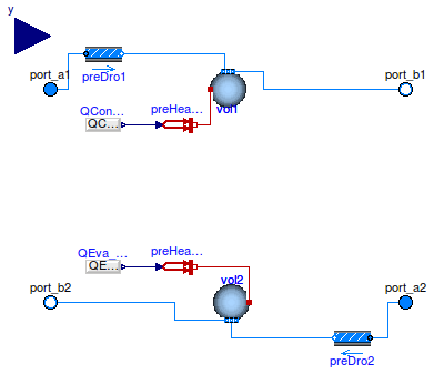
model Carnot 
  "Chiller with performance curve adjusted based on Carnot efficiency"
 extends Interfaces.FourPortHeatMassExchanger(final show_T = true,
    vol1(
      final prescribedHeatFlowRate = true),
    redeclare final Buildings.Fluid.MixingVolumes.MixingVolume vol2);

  parameter Buildings.Fluid.Types.EfficiencyInput effInpEva=
    Buildings.Fluid.Types.EfficiencyInput.volume 
    "Temperatures of evaporator fluid used to compute Carnot efficiency";
  parameter Buildings.Fluid.Types.EfficiencyInput effInpCon=
    Buildings.Fluid.Types.EfficiencyInput.port_a 
    "Temperatures of condenser fluid used to compute Carnot efficiency";
  parameter Modelica.SIunits.Power P_nominal 
    "Nominal compressor power (at y=1)";
  parameter Modelica.SIunits.TemperatureDifference dTEva_nominal = 10 
    "Temperature difference evaporator inlet-outlet";
  parameter Modelica.SIunits.TemperatureDifference dTCon_nominal = 10 
    "Temperature difference condenser outlet-inlet";
  // Efficiency
  parameter Boolean use_eta_Carnot = true 
    "Set to true to use Carnot efficiency";
  parameter Real etaCar(fixed=use_eta_Carnot) 
    "Carnot effectiveness (=COP/COP_Carnot)";
  parameter Real COP_nominal(fixed=not use_eta_Carnot) 
    "Coefficient of performance";
  parameter Modelica.SIunits.Temperature TCon_nominal = 303.15 
    "Condenser temperature";
  parameter Modelica.SIunits.Temperature TEva_nominal = 278.15 
    "Evaporator temperature";

  parameter Real a[:] = {1} 
    "Coefficients for efficiency curve (need p(a=a, y=1)=1)";

  Modelica.Blocks.Interfaces.RealInput y(min=0, max=1) "Part load ratio";
  Real etaPL "Efficiency due to part load of compressor (etaPL(y=1)=1";
  Real COP(min=0) "Coefficient of performance";
  Real COPCar(min=0) "Carnot efficiency";
  Modelica.SIunits.HeatFlowRate QCon_flow "Condenser heat input";
  Modelica.SIunits.HeatFlowRate QEva_flow "Evaporator heat input";
  Modelica.SIunits.Power P "Compressor power";
  Modelica.SIunits.Temperature TCon 
    "Condenser temperature used to compute efficiency";
  Modelica.SIunits.Temperature TEva 
    "Evaporator temperature used to compute efficiency";
protected 
  Buildings.HeatTransfer.Sources.PrescribedHeatFlow preHeaFloEva 
    "Prescribed heat flow rate";
  Buildings.HeatTransfer.Sources.PrescribedHeatFlow preHeaFloCon 
    "Prescribed heat flow rate";
  Modelica.Blocks.Sources.RealExpression QEva_flow_in(y=QEva_flow) 
    "Evaporator heat flow rate";
  Modelica.Blocks.Sources.RealExpression QCon_flow_in(y=QCon_flow) 
    "Condenser heat flow rate";
initial equation 
  assert(dTEva_nominal>0, "Parameter dTEva_nominal must be positive.");
  assert(dTCon_nominal>0, "Parameter dTCon_nominal must be positive.");
  if use_eta_Carnot then
    COP_nominal = etaCar * TEva_nominal/(TCon_nominal-TEva_nominal);
  else
    etaCar = COP_nominal / (TEva_nominal/(TCon_nominal-TEva_nominal));
  end if;
  assert(abs(Buildings.Utilities.Math.Functions.polynomial(
         a=a, x=y)-1) < 0.01, "Efficiency curve is wrong. Need etaPL(y=1)=1.");
  assert(etaCar > 0.1, "Parameters lead to etaCar < 0.1. Check parameters.");
  assert(etaCar < 1,   "Parameters lead to etaCar > 1. Check parameters.");
equation 
  // Set temperatures that will be used to compute Carnot efficiency
  if effInpCon == Buildings.Fluid.Types.EfficiencyInput.volume then
    TCon = vol1.heatPort.T;
  elseif effInpCon == Buildings.Fluid.Types.EfficiencyInput.port_a then
    TCon = Medium1.temperature(sta_a1);
  elseif effInpCon == Buildings.Fluid.Types.EfficiencyInput.port_b then
    TCon = Medium1.temperature(sta_b1);
  else
    TCon = 0.5 * (Medium1.temperature(sta_a1)+Medium1.temperature(sta_b1));
  end if;

  if effInpEva == Buildings.Fluid.Types.EfficiencyInput.volume then
    TEva = vol2.heatPort.T;
  elseif effInpEva == Buildings.Fluid.Types.EfficiencyInput.port_a then
    TEva = Medium2.temperature(sta_a2);
  elseif effInpEva == Buildings.Fluid.Types.EfficiencyInput.port_b then
    TEva = Medium2.temperature(sta_b2);
  else
    TEva = 0.5 * (Medium2.temperature(sta_a2)+Medium2.temperature(sta_b2));
  end if;

  etaPL  = Buildings.Utilities.Math.Functions.polynomial(a=a, x=y);
  P = y * P_nominal;
  COPCar = TEva / Buildings.Utilities.Math.Functions.smoothMax(x1=1, x2=TCon-TEva, deltaX=0.25);
  COP = etaCar * COPCar * etaPL;
  -QEva_flow = COP * P;
  QCon_flow = P - QEva_flow;

  connect(QCon_flow_in.y, preHeaFloCon.Q_flow);
  connect(preHeaFloCon.port, vol1.heatPort);
  connect(QEva_flow_in.y, preHeaFloEva.Q_flow);
  connect(preHeaFloEva.port, vol2.heatPort);
end Carnot;

Buildings.Fluid.Chillers.ElectricReformulatedEIR

Electric chiller based on the DOE-2.1 model, but with performance as a function of condenser leaving instead of entering temperature

Buildings.Fluid.Chillers.ElectricReformulatedEIR

Information

Model of an electric chiller, based on the model by Hydeman et al. (2002) that has been developed in the CoolTools project and that is implemented in EnergyPlus as the model Chiller:Electric:ReformulatedEIR. This empirical model is similar to Buildings.Fluid.Chillers.ElectricEIR. The difference is that to compute the performance, this model uses the condenser leaving temperature instead of the entering temperature, and it uses a bicubic polynomial to compute the part load performance.

This model uses three functions to predict capacity and power consumption:

A biquadratic function is used to predict cooling capacity as a function of condenser leaving and evaporator leaving fluid temperature.
A bicubic function is used to predict power input to cooling capacity ratio as a function of condenser leaving temperature and part load ratio.
A biquadratic functions is used to predict power input to cooling capacity ratio as a function of condenser leaving and evaporator leaving fluid temperature.

These curves are stored in the data record per and are available from Buildings.Fluid.Chillers.Data.ElectricReformulatedEIRChiller. Additional performance curves can be developed using two available techniques (Hydeman and Gillespie, 2002). The first technique is called the Least-squares Linear Regression method and is used when sufficient performance data exist to employ standard least-square linear regression techniques. The second technique is called Reference Curve Method and is used when insufficient performance data exist to apply linear regression techniques. A detailed description of both techniques can be found in Hydeman and Gillespie (2002).

The model takes as an input the set point for the leaving chilled water temperature, which is met if the chiller has sufficient capacity. Thus, the model has a built-in, ideal temperature control. The model has three tests on the part load ratio and the cycling ratio:

The test
```
  PLR1 =min(QEva_flow_set/QEva_flow_ava, per.PLRMax);
```
ensures that the chiller capacity does not exceed the chiller capacity specified by the parameter per.PLRMax.
The test
```
  CR = min(PLR1/per.PRLMin, 1.0);
```
computes a cycling ratio. This ratio expresses the fraction of time that a chiller would run if it were to cycle because its load is smaller than the minimal load at which it can operate. Note that this model continuously operates even if the part load ratio is below the minimum part load ratio. Its leaving evaporator and condenser temperature can therefore be considered as an average temperature between the modes where the compressor is off and on.
The test
```
  PLR2 = max(per.PLRMinUnl, PLR1);
```
computes the part load ratio of the compressor. The assumption is that for a part load ratio below per.PLRMinUnl, the chiller uses hot gas bypass to reduce the capacity, while the compressor power draw does not change.

The electric power only contains the power for the compressor, but not any power for pumps or fans.

The model can be parametrized to compute a transient or steady-state response. The transient response of the boiler is computed using a first order differential equation for the evaporator and condenser fluid volumes. The chiller outlet temperatures are equal to the temperatures of these lumped volumes.

References

Hydeman, M., N. Webb, P. Sreedharan, and S. Blanc. 2002. Development and Testing of a Reformulated Regression-Based Electric Chiller Model. ASHRAE Transactions, HI-02-18-2.
Hydeman, M. and K.L. Gillespie. 2002. Tools and Techniques to Calibrate Electric Chiller Component Models. ASHRAE Transactions, AC-02-9-1.

Extends from Buildings.Fluid.Chillers.BaseClasses.PartialElectric (Partial model for electric chiller based on the model in DOE-2, CoolTools and EnergyPlus).

Parameters

Type Name Default Description

replaceable package Medium1 PartialMedium Medium 1 in the component

replaceable package Medium2 PartialMedium Medium 2 in the component

Generic per Performance data

Nominal condition

MassFlowRate m1_flow_nominal mCon_flow_nominal Nominal mass flow rate [kg/s]

MassFlowRate m2_flow_nominal mEva_flow_nominal Nominal mass flow rate [kg/s]

Pressure dp1_nominal Pressure [Pa]

Pressure dp2_nominal Pressure [Pa]

Initialization

MassFlowRate m1_flow.start 0 Mass flow rate from port_a1 to port_b1 (m1_flow > 0 is design flow direction) [kg/s]

Pressure dp1.start 0 Pressure difference between port_a1 and port_b1 [Pa]

MassFlowRate m2_flow.start 0 Mass flow rate from port_a2 to port_b2 (m2_flow > 0 is design flow direction) [kg/s]

Pressure dp2.start 0 Pressure difference between port_a2 and port_b2 [Pa]

Real capFunT.start 1 Cooling capacity factor function of temperature curve

Real EIRFunT.start 1 Power input to cooling capacity ratio function of temperature curve

Real EIRFunPLR.start 1 Power input to cooling capacity ratio function of part load ratio

Real PLR1.start 1 Part load ratio

Real PLR2.start 1 Part load ratio

Real CR.start 1 Cycling ratio

Assumptions

Boolean allowFlowReversal1 system.allowFlowReversal = true to allow flow reversal in medium 1, false restricts to design direction (port_a -> port_b)

Boolean allowFlowReversal2 system.allowFlowReversal = true to allow flow reversal in medium 2, false restricts to design direction (port_a -> port_b)

Advanced

MassFlowRate m1_flow_small 1E-4*abs(m1_flow_nominal) Small mass flow rate for regularization of zero flow [kg/s]

MassFlowRate m2_flow_small 1E-4*abs(m2_flow_nominal) Small mass flow rate for regularization of zero flow [kg/s]

Boolean homotopyInitialization true = true, use homotopy method

Diagnostics

Boolean show_V_flow false = true, if volume flow rate at inflowing port is computed

Boolean show_T false = true, if actual temperature at port is computed (may lead to events)

Flow resistance

Medium 1

Boolean from_dp1 false = true, use m_flow = f(dp) else dp = f(m_flow)

Boolean linearizeFlowResistance1 false = true, use linear relation between m_flow and dp for any flow rate

Real deltaM1 0.1 Fraction of nominal flow rate where flow transitions to laminar

Medium 2

Boolean from_dp2 false = true, use m_flow = f(dp) else dp = f(m_flow)

Boolean linearizeFlowResistance2 false = true, use linear relation between m_flow and dp for any flow rate

Real deltaM2 0.1 Fraction of nominal flow rate where flow transitions to laminar

Dynamics

Nominal condition

Time tau1 30 Time constant at nominal flow [s]

Time tau2 30 Time constant at nominal flow [s]

Equations

Dynamics energyDynamics Modelica.Fluid.Types.Dynamic... Formulation of energy balance

Dynamics massDynamics energyDynamics Formulation of mass balance

Initialization

Medium 1

AbsolutePressure p1_start Medium1.p_default Start value of pressure [Pa]

Temperature T1_start 273.15 + 25 Start value of temperature [K]

MassFraction X1_start[Medium1.nX] Medium1.X_default Start value of mass fractions m_i/m [kg/kg]

ExtraProperty C1_start[Medium1.nC] fill(0, Medium1.nC) Start value of trace substances

ExtraProperty C1_nominal[Medium1.nC] fill(1E-2, Medium1.nC) Nominal value of trace substances. (Set to typical order of magnitude.)

Medium 2

AbsolutePressure p2_start Medium2.p_default Start value of pressure [Pa]

Temperature T2_start 273.15 + 5 Start value of temperature [K]

MassFraction X2_start[Medium2.nX] Medium2.X_default Start value of mass fractions m_i/m [kg/kg]

ExtraProperty C2_start[Medium2.nC] fill(0, Medium2.nC) Start value of trace substances

ExtraProperty C2_nominal[Medium2.nC] fill(1E-2, Medium2.nC) Nominal value of trace substances. (Set to typical order of magnitude.)

Type	Name	Default	Description
replaceable package Medium1	PartialMedium	Medium 1 in the component
replaceable package Medium2	PartialMedium	Medium 2 in the component
Generic	per		Performance data
Nominal condition
MassFlowRate	m1_flow_nominal	mCon_flow_nominal	Nominal mass flow rate [kg/s]
MassFlowRate	m2_flow_nominal	mEva_flow_nominal	Nominal mass flow rate [kg/s]
Pressure	dp1_nominal		Pressure [Pa]
Pressure	dp2_nominal		Pressure [Pa]
Initialization
MassFlowRate	m1_flow.start	0	Mass flow rate from port_a1 to port_b1 (m1_flow > 0 is design flow direction) [kg/s]
Pressure	dp1.start	0	Pressure difference between port_a1 and port_b1 [Pa]
MassFlowRate	m2_flow.start	0	Mass flow rate from port_a2 to port_b2 (m2_flow > 0 is design flow direction) [kg/s]
Pressure	dp2.start	0	Pressure difference between port_a2 and port_b2 [Pa]
Real	capFunT.start	1	Cooling capacity factor function of temperature curve
Real	EIRFunT.start	1	Power input to cooling capacity ratio function of temperature curve
Real	EIRFunPLR.start	1	Power input to cooling capacity ratio function of part load ratio
Real	PLR1.start	1	Part load ratio
Real	PLR2.start	1	Part load ratio
Real	CR.start	1	Cycling ratio
Assumptions
Boolean	allowFlowReversal1	system.allowFlowReversal	= true to allow flow reversal in medium 1, false restricts to design direction (port_a -> port_b)
Boolean	allowFlowReversal2	system.allowFlowReversal	= true to allow flow reversal in medium 2, false restricts to design direction (port_a -> port_b)
Advanced
MassFlowRate	m1_flow_small	1E-4*abs(m1_flow_nominal)	Small mass flow rate for regularization of zero flow [kg/s]
MassFlowRate	m2_flow_small	1E-4*abs(m2_flow_nominal)	Small mass flow rate for regularization of zero flow [kg/s]
Boolean	homotopyInitialization	true	= true, use homotopy method
Diagnostics
Boolean	show_V_flow	false	= true, if volume flow rate at inflowing port is computed
Boolean	show_T	false	= true, if actual temperature at port is computed (may lead to events)
Flow resistance
Medium 1
Boolean	from_dp1	false	= true, use m_flow = f(dp) else dp = f(m_flow)
Boolean	linearizeFlowResistance1	false	= true, use linear relation between m_flow and dp for any flow rate
Real	deltaM1	0.1	Fraction of nominal flow rate where flow transitions to laminar
Medium 2
Boolean	from_dp2	false	= true, use m_flow = f(dp) else dp = f(m_flow)
Boolean	linearizeFlowResistance2	false	= true, use linear relation between m_flow and dp for any flow rate
Real	deltaM2	0.1	Fraction of nominal flow rate where flow transitions to laminar
Dynamics
Nominal condition
Time	tau1	30	Time constant at nominal flow [s]
Time	tau2	30	Time constant at nominal flow [s]
Equations
Dynamics	energyDynamics	Modelica.Fluid.Types.Dynamic...	Formulation of energy balance
Dynamics	massDynamics	energyDynamics	Formulation of mass balance
Initialization
Medium 1
AbsolutePressure	p1_start	Medium1.p_default	Start value of pressure [Pa]
Temperature	T1_start	273.15 + 25	Start value of temperature [K]
MassFraction	X1_start[Medium1.nX]	Medium1.X_default	Start value of mass fractions m_i/m [kg/kg]
ExtraProperty	C1_start[Medium1.nC]	fill(0, Medium1.nC)	Start value of trace substances
ExtraProperty	C1_nominal[Medium1.nC]	fill(1E-2, Medium1.nC)	Nominal value of trace substances. (Set to typical order of magnitude.)
Medium 2
AbsolutePressure	p2_start	Medium2.p_default	Start value of pressure [Pa]
Temperature	T2_start	273.15 + 5	Start value of temperature [K]
MassFraction	X2_start[Medium2.nX]	Medium2.X_default	Start value of mass fractions m_i/m [kg/kg]
ExtraProperty	C2_start[Medium2.nC]	fill(0, Medium2.nC)	Start value of trace substances
ExtraProperty	C2_nominal[Medium2.nC]	fill(1E-2, Medium2.nC)	Nominal value of trace substances. (Set to typical order of magnitude.)

Connectors

Type	Name	Description
FluidPort_a	port_a1	Fluid connector a1 (positive design flow direction is from port_a1 to port_b1)
FluidPort_b	port_b1	Fluid connector b1 (positive design flow direction is from port_a1 to port_b1)
FluidPort_a	port_a2	Fluid connector a2 (positive design flow direction is from port_a2 to port_b2)
FluidPort_b	port_b2	Fluid connector b2 (positive design flow direction is from port_a2 to port_b2)
input BooleanInput	on	Set to true to enable compressor, or false to disable compressor
input RealInput	TSet	Set point for leaving chilled water temperature [K]
output RealOutput	P	Electric power consumed by compressor [W]

Modelica definition

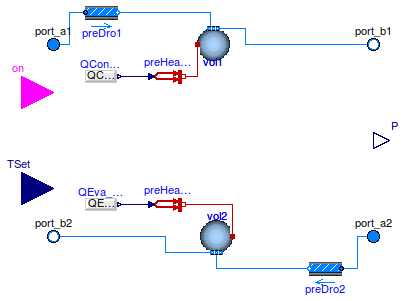
model ElectricReformulatedEIR 
  "Electric chiller based on the DOE-2.1 model, but with performance as a function of condenser leaving instead of entering temperature"
  extends Buildings.Fluid.Chillers.BaseClasses.PartialElectric(
  final QEva_flow_nominal = per.QEva_flow_nominal,
  final COP_nominal= per.COP_nominal,
  final PLRMax= per.PLRMax,
  final PLRMinUnl= per.PLRMinUnl,
  final PLRMin= per.PLRMin,
  final etaMotor= per.etaMotor,
  final mEva_flow_nominal= per.mEva_flow_nominal,
  final mCon_flow_nominal= per.mCon_flow_nominal,
  final TEvaLvg_nominal= per.TEvaLvg_nominal);

  parameter Buildings.Fluid.Chillers.Data.ElectricReformulatedEIR.Generic per 
    "Performance data";

protected 
  final parameter Modelica.SIunits.Conversions.NonSIunits.Temperature_degC
    TConLvg_nominal_degC=
    Modelica.SIunits.Conversions.to_degC(per.TConLvg_nominal) 
    "Temperature of fluid leaving condenser at nominal condition";

  Modelica.SIunits.Conversions.NonSIunits.Temperature_degC TConLvg_degC 
    "Temperature of fluid leaving condenser";
initial equation 
  // Verify correctness of performance curves, and write warning if error is bigger than 10%
  Buildings.Fluid.Chillers.BaseClasses.warnIfPerformanceOutOfBounds(
     Buildings.Utilities.Math.Functions.biquadratic(a=per.capFunT,
     x1=TEvaLvg_nominal_degC, x2=TConLvg_nominal_degC),
     "Capacity as function of temperature ",
     "per.capFunT");
equation 
  TConLvg_degC=Modelica.SIunits.Conversions.to_degC(TConLvg);

  if on then
    // Compute the chiller capacity fraction, using a biquadratic curve.
    // Since the regression for capacity can have negative values (for unreasonable temperatures),
    // we constrain its return value to be non-negative. This prevents the solver to pick the
    // unrealistic solution.
    capFunT = max(0,
       Buildings.Utilities.Math.Functions.biquadratic(a=per.capFunT, x1=TEvaLvg_degC, x2=TConLvg_degC));
/*    assert(capFunT > 0.1, "Error: Received capFunT = " + String(capFunT)  + ".\n"
           + "Coefficient for polynomial seem to be not valid for the encountered temperature range.\n"
           + "Temperatures are TConLvg_degC = " + String(TConLvg_degC) + " degC\n"
           + "                 TEvaLvg_degC = " + String(TEvaLvg_degC) + " degC");
*/
    // Chiller energy input ratio biquadratic curve.
    EIRFunT = Buildings.Utilities.Math.Functions.biquadratic(a=per.EIRFunT, x1=TEvaLvg_degC, x2=TConLvg_degC);
    // Chiller energy input ratio bicubic curve
    EIRFunPLR   = Buildings.Utilities.Math.Functions.bicubic(a=per.EIRFunPLR, x1=TConLvg_degC, x2=PLR2);
  else
    capFunT   = 0;
    EIRFunT   = 0;
    EIRFunPLR = 0;
  end if;
end ElectricReformulatedEIR;

Buildings.Fluid.Chillers.ElectricEIR

Electric chiller based on the DOE-2.1 model

Buildings.Fluid.Chillers.ElectricEIR

Information

Model of an electric chiller, based on the DOE-2.1 chiller model and the EnergyPlus chiller model Chiller:Electric:EIR.

This model uses three functions to predict capacity and power consumption:

A biquadratic function is used to predict cooling capacity as a function of condenser entering and evaporator leaving fluid temperature.
A quadratic functions is used to predict power input to cooling capacity ratio with respect to the part load ratio.
A biquadratic functions is used to predict power input to cooling capacity ratio as a function of condenser entering and evaporator leaving fluid temperature.

These curves are stored in the data record per and are available from Buildings.Fluid.Chillers.Data.ElectricEIR. Additional performance curves can be developed using two available techniques (Hydeman and Gillespie, 2002). The first technique is called the Least-squares Linear Regression method and is used when sufficient performance data exist to employ standard least-square linear regression techniques. The second technique is called Reference Curve Method and is used when insufficient performance data exist to apply linear regression techniques. A detailed description of both techniques can be found in Hydeman and Gillespie (2002).

The test
```
  PLR1 =min(QEva_flow_set/QEva_flow_ava, per.PLRMax);
```
ensures that the chiller capacity does not exceed the chiller capacity specified by the parameter per.PLRMax.
The test
```
  CR = min(PLR1/per.PRLMin, 1.0);
```
computes a cycling ratio. This ratio expresses the fraction of time that a chiller would run if it were to cycle because its load is smaller than the minimal load at which it can operate. Note that this model continuously operates even if the part load ratio is below the minimum part load ratio. Its leaving evaporator and condenser temperature can therefore be considered as an average temperature between the modes where the compressor is off and on.
The test
```
  PLR2 = max(per.PLRMinUnl, PLR1);
```
computes the part load ratio of the compressor. The assumption is that for a part load ratio below per.PLRMinUnl, the chiller uses hot gas bypass to reduce the capacity, while the compressor power draw does not change.

The electric power only contains the power for the compressor, but not any power for pumps or fans.

References

Hydeman, M. and K.L. Gillespie. 2002. Tools and Techniques to Calibrate Electric Chiller Component Models. ASHRAE Transactions, AC-02-9-1.

Extends from Buildings.Fluid.Chillers.BaseClasses.PartialElectric (Partial model for electric chiller based on the model in DOE-2, CoolTools and EnergyPlus).

Parameters

Type	Name	Default	Description
replaceable package Medium1	PartialMedium	Medium 1 in the component
replaceable package Medium2	PartialMedium	Medium 2 in the component
Generic	per		Performance data
Nominal condition
MassFlowRate	m1_flow_nominal	mCon_flow_nominal	Nominal mass flow rate [kg/s]
MassFlowRate	m2_flow_nominal	mEva_flow_nominal	Nominal mass flow rate [kg/s]
Pressure	dp1_nominal		Pressure [Pa]
Pressure	dp2_nominal		Pressure [Pa]
Initialization
MassFlowRate	m1_flow.start	0	Mass flow rate from port_a1 to port_b1 (m1_flow > 0 is design flow direction) [kg/s]
Pressure	dp1.start	0	Pressure difference between port_a1 and port_b1 [Pa]
MassFlowRate	m2_flow.start	0	Mass flow rate from port_a2 to port_b2 (m2_flow > 0 is design flow direction) [kg/s]
Pressure	dp2.start	0	Pressure difference between port_a2 and port_b2 [Pa]
Real	capFunT.start	1	Cooling capacity factor function of temperature curve
Real	EIRFunT.start	1	Power input to cooling capacity ratio function of temperature curve
Real	EIRFunPLR.start	1	Power input to cooling capacity ratio function of part load ratio
Real	PLR1.start	1	Part load ratio
Real	PLR2.start	1	Part load ratio
Real	CR.start	1	Cycling ratio
Assumptions
Boolean	allowFlowReversal1	system.allowFlowReversal	= true to allow flow reversal in medium 1, false restricts to design direction (port_a -> port_b)
Boolean	allowFlowReversal2	system.allowFlowReversal	= true to allow flow reversal in medium 2, false restricts to design direction (port_a -> port_b)
Advanced
MassFlowRate	m1_flow_small	1E-4*abs(m1_flow_nominal)	Small mass flow rate for regularization of zero flow [kg/s]
MassFlowRate	m2_flow_small	1E-4*abs(m2_flow_nominal)	Small mass flow rate for regularization of zero flow [kg/s]
Boolean	homotopyInitialization	true	= true, use homotopy method
Diagnostics
Boolean	show_V_flow	false	= true, if volume flow rate at inflowing port is computed
Boolean	show_T	false	= true, if actual temperature at port is computed (may lead to events)
Flow resistance
Medium 1
Boolean	from_dp1	false	= true, use m_flow = f(dp) else dp = f(m_flow)
Boolean	linearizeFlowResistance1	false	= true, use linear relation between m_flow and dp for any flow rate
Real	deltaM1	0.1	Fraction of nominal flow rate where flow transitions to laminar
Medium 2
Boolean	from_dp2	false	= true, use m_flow = f(dp) else dp = f(m_flow)
Boolean	linearizeFlowResistance2	false	= true, use linear relation between m_flow and dp for any flow rate
Real	deltaM2	0.1	Fraction of nominal flow rate where flow transitions to laminar
Dynamics
Nominal condition
Time	tau1	30	Time constant at nominal flow [s]
Time	tau2	30	Time constant at nominal flow [s]
Equations
Dynamics	energyDynamics	Modelica.Fluid.Types.Dynamic...	Formulation of energy balance
Dynamics	massDynamics	energyDynamics	Formulation of mass balance
Initialization
Medium 1
AbsolutePressure	p1_start	Medium1.p_default	Start value of pressure [Pa]
Temperature	T1_start	273.15 + 25	Start value of temperature [K]
MassFraction	X1_start[Medium1.nX]	Medium1.X_default	Start value of mass fractions m_i/m [kg/kg]
ExtraProperty	C1_start[Medium1.nC]	fill(0, Medium1.nC)	Start value of trace substances
ExtraProperty	C1_nominal[Medium1.nC]	fill(1E-2, Medium1.nC)	Nominal value of trace substances. (Set to typical order of magnitude.)
Medium 2
AbsolutePressure	p2_start	Medium2.p_default	Start value of pressure [Pa]
Temperature	T2_start	273.15 + 5	Start value of temperature [K]
MassFraction	X2_start[Medium2.nX]	Medium2.X_default	Start value of mass fractions m_i/m [kg/kg]
ExtraProperty	C2_start[Medium2.nC]	fill(0, Medium2.nC)	Start value of trace substances
ExtraProperty	C2_nominal[Medium2.nC]	fill(1E-2, Medium2.nC)	Nominal value of trace substances. (Set to typical order of magnitude.)

Connectors

Type	Name	Description
FluidPort_a	port_a1	Fluid connector a1 (positive design flow direction is from port_a1 to port_b1)
FluidPort_b	port_b1	Fluid connector b1 (positive design flow direction is from port_a1 to port_b1)
FluidPort_a	port_a2	Fluid connector a2 (positive design flow direction is from port_a2 to port_b2)
FluidPort_b	port_b2	Fluid connector b2 (positive design flow direction is from port_a2 to port_b2)
input BooleanInput	on	Set to true to enable compressor, or false to disable compressor
input RealInput	TSet	Set point for leaving chilled water temperature [K]
output RealOutput	P	Electric power consumed by compressor [W]

Modelica definition

model ElectricEIR "Electric chiller based on the DOE-2.1 model"
  extends Buildings.Fluid.Chillers.BaseClasses.PartialElectric(
  final QEva_flow_nominal = per.QEva_flow_nominal,
  final COP_nominal= per.COP_nominal,
  final PLRMax= per.PLRMax,
  final PLRMinUnl= per.PLRMinUnl,
  final PLRMin= per.PLRMin,
  final etaMotor= per.etaMotor,
  final mEva_flow_nominal= per.mEva_flow_nominal,
  final mCon_flow_nominal= per.mCon_flow_nominal,
  final TEvaLvg_nominal= per.TEvaLvg_nominal);

  parameter Buildings.Fluid.Chillers.Data.ElectricEIR.Generic per 
    "Performance data";

protected 
  final parameter Modelica.SIunits.Conversions.NonSIunits.Temperature_degC
    TConEnt_nominal_degC=
    Modelica.SIunits.Conversions.to_degC(per.TConEnt_nominal) 
    "Temperature of fluid entering condenser at nominal condition";

  Modelica.SIunits.Conversions.NonSIunits.Temperature_degC TConEnt_degC 
    "Temperature of fluid entering condenser";
initial equation 
  // Verify correctness of performance curves, and write warning if error is bigger than 10%
  Buildings.Fluid.Chillers.BaseClasses.warnIfPerformanceOutOfBounds(
     Buildings.Utilities.Math.Functions.biquadratic(a=per.capFunT,
     x1=TEvaLvg_nominal_degC, x2=TConEnt_nominal_degC),
     "Capacity as function of temperature ",
     "per.capFunT");
equation 
  TConEnt_degC=Modelica.SIunits.Conversions.to_degC(TConEnt);

  if on then
    // Compute the chiller capacity fraction, using a biquadratic curve.
    // Since the regression for capacity can have negative values (for unreasonable temperatures),
    // we constrain its return value to be non-negative. This prevents the solver to pick the
    // unrealistic solution.
    capFunT = max(0,
       Buildings.Utilities.Math.Functions.biquadratic(a=per.capFunT, x1=TEvaLvg_degC, x2=TConEnt_degC));
/*    assert(capFunT > 0.1, "Error: Received capFunT = " + String(capFunT)  + ".\n"
           + "Coefficient for polynomial seem to be not valid for the encountered temperature range.\n"
           + "Temperatures are TConEnt_degC = " + String(TConEnt_degC) + " degC\n"
           + "                 TEvaLvg_degC = " + String(TEvaLvg_degC) + " degC");
*/
    // Chiller energy input ratio biquadratic curve.
    EIRFunT = Buildings.Utilities.Math.Functions.biquadratic(a=per.EIRFunT, x1=TEvaLvg_degC, x2=TConEnt_degC);
    // Chiller energy input ratio quadratic curve
    EIRFunPLR   = per.EIRFunPLR[1]+per.EIRFunPLR[2]*PLR2+per.EIRFunPLR[3]*PLR2^2;
  else
    capFunT   = 0;
    EIRFunT   = 0;
    EIRFunPLR = 0;
  end if;

end ElectricEIR;

Automatically generated Thu Jul 26 10:20:20 2012.