This package contains basic continuous input/output blocks described by differential equations.
All blocks of this package can be initialized in different ways controlled by parameter initType. The possible values of initType are defined in Modelica.Blocks.Types.Init:
| Name | Description |
| Init.NoInit | no initialization (start values are used as guess values with fixed=false) |
| Init.SteadyState | steady state initialization (derivatives of states are zero) |
| Init.InitialState | Initialization with initial states |
| Init.InitialOutput | Initialization with initial outputs (and steady state of the states if possibles) |
For backward compatibility reasons the default of all blocks is Init.NoInit, with the exception of Integrator and LimIntegrator where the default is Init.InitialState (this was the initialization defined in version 2.2 of the Modelica standard library).
In many cases, the most useful initial condition is Init.SteadyState because initial transients are then no longer present. The drawback is that in combination with a non-linear plant, non-linear algebraic equations occur that might be difficult to solve if appropriate guess values for the iteration variables are not provided (i.e., start values with fixed=false). However, it is often already useful to just initialize the linear blocks from the Continuous blocks library in SteadyState. This is uncritical, because only linear algebraic equations occur. If Init.NoInit is set, then the start values for the states are interpreted as guess values and are propagated to the states with fixed=false.
Note, initialization with Init.SteadyState is usually difficult for a block that contains an integrator (Integrator, LimIntegrator, PI, PID, LimPID). This is due to the basic equation of an integrator:
  initial equation
     der(y) = 0;   // Init.SteadyState
  equation
     der(y) = k*u;
The steady state equation leads to the condition that the input to the integrator is zero. If the input u is already (directly or indirectly) defined by another initial condition, then the initialization problem is singular (has none or infinitely many solutions). This situation occurs often for mechanical systems, where, e.g., u = desiredSpeed - measuredSpeed and since speed is both a state and a derivative, it is always defined by Init.InitialState or Init.SteadyState initializtion.
In such a case, Init.NoInit has to be selected for the integrator and an additional initial equation has to be added to the system to which the integrator is connected. E.g., useful initial conditions for a 1-dim. rotational inertia controlled by a PI controller are that angle, speed, and acceleration of the inertia are zero.
Extends from Modelica.Icons.Package (Icon for standard packages).
| Name | Description |
|---|---|
| Output the integral of the input signal | |
| Integrator with limited value of the output | |
| Approximated derivative block | |
| First order transfer function block (= 1 pole) | |
| Second order transfer function block (= 2 poles) | |
| Proportional-Integral controller | |
| PID-controller in additive description form | |
| P, PI, PD, and PID controller with limited output, anti-windup compensation and setpoint weighting | |
| Linear transfer function | |
| Linear state space system | |
| Derivative of input (= analytic differentations) | |
| Output the input signal filtered with a low pass Butterworth filter of any order | |
| Output the input signal filtered with an n-th order filter with critical damping | |
| Continuous low pass, high pass, band pass or band stop IIR-filter of type CriticalDamping, Bessel, Butterworth or ChebyshevI | |
| Internal utility functions and blocks that should not be directly utilized by the user |
 Modelica.Blocks.Continuous.Integrator
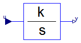
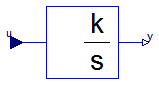
This blocks computes output y (element-wise) as integral of the input u multiplied with the gain k:
         k
     y = - u
         s
It might be difficult to initialize the integrator in steady state. This is discussed in the description of package Continuous.
Extends from Interfaces.SISO (Single Input Single Output continuous control block).
| Type | Name | Default | Description |
|---|---|---|---|
| Real | k | 1 | Integrator gain [1] |
| Initialization | |||
| Init | initType | Modelica.Blocks.Types.Init.I... | Type of initialization (1: no init, 2: steady state, 3,4: initial output) |
| Real | y_start | 0 | Initial or guess value of output (= state) |
| RealOutput | y.start | y_start | Connector of Real output signal |
| Type | Name | Description |
|---|---|---|
| input RealInput | u | Connector of Real input signal |
block Integrator "Output the integral of the input signal"
  import Modelica.Blocks.Types.Init;
  parameter Real k(unit="1")=1 "Integrator gain";

  /* InitialState is the default, because it was the default in Modelica 2.2
     and therefore this setting is backward compatible
  */
  parameter Modelica.Blocks.Types.Init initType=Modelica.Blocks.Types.Init.InitialState
    "Type of initialization (1: no init, 2: steady state, 3,4: initial output)";
  parameter Real y_start=0 "Initial or guess value of output (= state)";
  extends Interfaces.SISO(y(start=y_start));

initial equation
  if initType == Init.SteadyState then
     der(y) = 0;
  elseif initType == Init.InitialState or
         initType == Init.InitialOutput then
    y = y_start;
  end if;
equation
  der(y) = k*u;
end Integrator;
 Modelica.Blocks.Continuous.LimIntegrator
This blocks computes y (element-wise) as integral of the input u multiplied with the gain k. If the integral reaches a given upper or lower limit and the input will drive the integral outside of this bound, the integration is halted and only restarted if the input drives the integral away from the bounds.
It might be difficult to initialize the integrator in steady state. This is discussed in the description of package Continuous.
If parameter limitAtInit = false, the limits of the integrator are removed from the initialization problem which leads to a much simpler equation system. After initialization has been performed, it is checked via an assert whether the output is in the defined limits. For backward compatibility reasons limitAtInit = true. In most cases it is best to use limitAtInit = false.
Extends from Interfaces.SISO (Single Input Single Output continuous control block).
| Type | Name | Default | Description |
|---|---|---|---|
| Real | k | 1 | Integrator gain [1] |
| Real | outMax | Upper limit of output | |
| Real | outMin | -outMax | Lower limit of output |
| Initialization | |||
| Init | initType | Modelica.Blocks.Types.Init.I... | Type of initialization (1: no init, 2: steady state, 3/4: initial output) |
| Boolean | limitsAtInit | true | = false, if limits are ignored during initializiation (i.e., der(y)=k*u) |
| Real | y_start | 0 | Initial or guess value of output (must be in the limits outMin .. outMax) |
| RealOutput | y.start | y_start | Connector of Real output signal |
| Type | Name | Description |
|---|---|---|
| input RealInput | u | Connector of Real input signal |
block LimIntegrator "Integrator with limited value of the output"
  import Modelica.Blocks.Types.Init;
  parameter Real k(unit="1")=1 "Integrator gain";
  parameter Real outMax(start=1) "Upper limit of output";
  parameter Real outMin=-outMax "Lower limit of output";
  parameter Modelica.Blocks.Types.Init initType=Modelica.Blocks.Types.Init.InitialState
    "Type of initialization (1: no init, 2: steady state, 3/4: initial output)";
  parameter Boolean limitsAtInit = true
    "= false, if limits are ignored during initializiation (i.e., der(y)=k*u)";
  parameter Real y_start=0
    "Initial or guess value of output (must be in the limits outMin .. outMax)";
  extends Interfaces.SISO(y(start=y_start));

initial equation
  if initType == Init.SteadyState then
     der(y) = 0;
  elseif initType == Init.InitialState or
         initType == Init.InitialOutput then
    y = y_start;
  end if;
equation
  if initial() and not limitsAtInit then
     der(y) = k*u;
     assert(y >= outMin - 0.01*abs(outMin) and
            y <= outMax + 0.01*abs(outMax),
           "LimIntegrator: During initialization the limits have been ignored.\n"+
           "However, the result is that the output y is not within the required limits:\n"+
           "  y = " + String(y) + ", outMin = " + String(outMin) + ", outMax = " + String(outMax));
  else
     der(y) = if y < outMin and u < 0 or y > outMax and u > 0 then 0 else k*u;
  end if;
end LimIntegrator;
 Modelica.Blocks.Continuous.Derivative
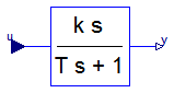
This blocks defines the transfer function between the input u and the output y (element-wise) as approximated derivative:
             k * s
     y = ------------ * u
            T * s + 1
If you would like to be able to change easily between different
transfer functions (FirstOrder, SecondOrder, ... ) by changing
parameters, use the general block TransferFunction instead
and model a derivative block with parameters
b = {k,0}, a = {T, 1}.
If k=0, the block reduces to y=0.
Extends from Interfaces.SISO (Single Input Single Output continuous control block).
| Type | Name | Default | Description |
|---|---|---|---|
| Real | k | 1 | Gains [1] |
| Time | T | 0.01 | Time constants (T>0 required; T=0 is ideal derivative block) [s] |
| Initialization | |||
| Init | initType | Modelica.Blocks.Types.Init.N... | Type of initialization (1: no init, 2: steady state, 3: initial state, 4: initial output) |
| Real | x_start | 0 | Initial or guess value of state |
| Real | y_start | 0 | Initial value of output (= state) |
| Type | Name | Description |
|---|---|---|
| input RealInput | u | Connector of Real input signal |
| output RealOutput | y | Connector of Real output signal |
block Derivative "Approximated derivative block"
  import Modelica.Blocks.Types.Init;
  parameter Real k(unit="1")=1 "Gains";
  parameter SIunits.Time T(min=Modelica.Constants.small) = 0.01
    "Time constants (T>0 required; T=0 is ideal derivative block)";
  parameter Modelica.Blocks.Types.Init initType=Modelica.Blocks.Types.Init.NoInit
    "Type of initialization (1: no init, 2: steady state, 3: initial state, 4: initial output)";
  parameter Real x_start=0 "Initial or guess value of state";
  parameter Real y_start=0 "Initial value of output (= state)";
  extends Interfaces.SISO;

  output Real x(start=x_start) "State of block";

protected
  parameter Boolean zeroGain = abs(k) < Modelica.Constants.eps;
initial equation
  if initType == Init.SteadyState then
    der(x) = 0;
  elseif initType == Init.InitialState then
    x = x_start;
  elseif initType == Init.InitialOutput then
    if zeroGain then
       x = u;
    else
       y = y_start;
    end if;
  end if;
equation
  der(x) = if zeroGain then 0 else (u - x)/T;
  y = if zeroGain then 0 else (k/T)*(u - x);
end Derivative;
 Modelica.Blocks.Continuous.FirstOrder
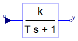
This blocks defines the transfer function between the input u and the output y (element-wise) as first order system:
               k
     y = ------------ * u
            T * s + 1
If you would like to be able to change easily between different
transfer functions (FirstOrder, SecondOrder, ... ) by changing
parameters, use the general block TransferFunction instead
and model a first order SISO system with parameters
b = {k}, a = {T, 1}.
Example:
   parameter: k = 0.3, T = 0.4
   results in:
             0.3
      y = ----------- * u
          0.4 s + 1.0
Extends from Interfaces.SISO (Single Input Single Output continuous control block).
| Type | Name | Default | Description |
|---|---|---|---|
| Real | k | 1 | Gain [1] |
| Time | T | Time Constant [s] | |
| Initialization | |||
| Init | initType | Modelica.Blocks.Types.Init.N... | Type of initialization (1: no init, 2: steady state, 3/4: initial output) |
| Real | y_start | 0 | Initial or guess value of output (= state) |
| RealOutput | y.start | y_start | Connector of Real output signal |
| Type | Name | Description |
|---|---|---|
| input RealInput | u | Connector of Real input signal |
block FirstOrder "First order transfer function block (= 1 pole)"
  import Modelica.Blocks.Types.Init;
  parameter Real k(unit="1")=1 "Gain";
  parameter SIunits.Time T(start=1) "Time Constant";
  parameter Modelica.Blocks.Types.Init initType=Modelica.Blocks.Types.Init.NoInit
    "Type of initialization (1: no init, 2: steady state, 3/4: initial output)";
  parameter Real y_start=0 "Initial or guess value of output (= state)";

  extends Interfaces.SISO(y(start=y_start));

initial equation
  if initType == Init.SteadyState then
    der(y) = 0;
  elseif initType == Init.InitialState or initType == Init.InitialOutput then
    y = y_start;
  end if;
equation
  der(y) = (k*u - y)/T;
end FirstOrder;
 Modelica.Blocks.Continuous.SecondOrder
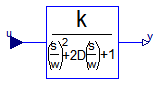
This blocks defines the transfer function between the input u and the output y (element-wise) as second order system:
                             k
     y = ---------------------------------------- * u
            ( s / w )^2 + 2*D*( s / w ) + 1
If you would like to be able to change easily between different
transfer functions (FirstOrder, SecondOrder, ... ) by changing
parameters, use the general model class TransferFunction
instead and model a second order SISO system with parameters
b = {k}, a = {1/w^2, 2*D/w, 1}.
Example:

   parameter: k =  0.3,  w = 0.5,  D = 0.4
   results in:
                  0.3
      y = ------------------- * u
          4.0 s^2 + 1.6 s + 1
Extends from Interfaces.SISO (Single Input Single Output continuous control block).
| Type | Name | Default | Description |
|---|---|---|---|
| Real | k | 1 | Gain [1] |
| Real | w | Angular frequency | |
| Real | D | Damping | |
| Initialization | |||
| Init | initType | Modelica.Blocks.Types.Init.N... | Type of initialization (1: no init, 2: steady state, 3/4: initial output) |
| Real | y_start | 0 | Initial or guess value of output (= state) |
| Real | yd_start | 0 | Initial or guess value of derivative of output (= state) |
| RealOutput | y.start | y_start | Connector of Real output signal |
| Type | Name | Description |
|---|---|---|
| input RealInput | u | Connector of Real input signal |
block SecondOrder "Second order transfer function block (= 2 poles)"
  import Modelica.Blocks.Types.Init;
  parameter Real k(unit="1")=1 "Gain";
  parameter Real w(start=1) "Angular frequency";
  parameter Real D(start=1) "Damping";
  parameter Modelica.Blocks.Types.Init initType=Modelica.Blocks.Types.Init.NoInit
    "Type of initialization (1: no init, 2: steady state, 3/4: initial output)";
  parameter Real y_start=0 "Initial or guess value of output (= state)";
  parameter Real yd_start=0
    "Initial or guess value of derivative of output (= state)";

  extends Interfaces.SISO(y(start=y_start));
  output Real yd(start=yd_start) "Derivative of y";

initial equation
  if initType == Init.SteadyState then
    der(y) = 0;
    der(yd) = 0;
  elseif initType == Init.InitialState or initType == Init.InitialOutput then
    y = y_start;
    yd = yd_start;
  end if;
equation
  der(y) = yd;
  der(yd) = w*(w*(k*u - y) - 2*D*yd);
end SecondOrder;
 Modelica.Blocks.Continuous.PI
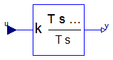
This blocks defines the transfer function between the input u and the output y (element-wise) as PI system:
                 1
   y = k * (1 + ---) * u
                T*s
           T*s + 1
     = k * ------- * u
             T*s
If you would like to be able to change easily between different
transfer functions (FirstOrder, SecondOrder, ... ) by changing
parameters, use the general model class TransferFunction
instead and model a PI SISO system with parameters
b = {k*T, k}, a = {T, 0}.
Example:

   parameter: k = 0.3,  T = 0.4

   results in:
               0.4 s + 1
      y = 0.3 ----------- * u
                 0.4 s
It might be difficult to initialize the PI component in steady state due to the integrator part. This is discussed in the description of package Continuous.
Extends from Interfaces.SISO (Single Input Single Output continuous control block).
| Type | Name | Default | Description |
|---|---|---|---|
| Real | k | 1 | Gain [1] |
| Time | T | Time Constant (T>0 required) [s] | |
| Initialization | |||
| Init | initType | Modelica.Blocks.Types.Init.N... | Type of initialization (1: no init, 2: steady state, 3: initial state, 4: initial output) |
| Real | x_start | 0 | Initial or guess value of state |
| Real | y_start | 0 | Initial value of output |
| Type | Name | Description |
|---|---|---|
| input RealInput | u | Connector of Real input signal |
| output RealOutput | y | Connector of Real output signal |
block PI "Proportional-Integral controller"
  import Modelica.Blocks.Types.Init;
  parameter Real k(unit="1")=1 "Gain";
  parameter SIunits.Time T(start=1,min=Modelica.Constants.small)
    "Time Constant (T>0 required)";
  parameter Modelica.Blocks.Types.Init initType=Modelica.Blocks.Types.Init.NoInit
    "Type of initialization (1: no init, 2: steady state, 3: initial state, 4: initial output)";
  parameter Real x_start=0 "Initial or guess value of state";
  parameter Real y_start=0 "Initial value of output";

  extends Interfaces.SISO;
  output Real x(start=x_start) "State of block";

initial equation
  if initType == Init.SteadyState then
    der(x) = 0;
  elseif initType == Init.InitialState then
    x = x_start;
  elseif initType == Init.InitialOutput then
    y = y_start;
  end if;
equation
  der(x) = u/T;
  y = k*(x + u);
end PI;
 Modelica.Blocks.Continuous.PID
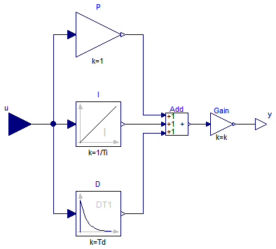
This is the text-book version of a PID-controller. For a more practically useful PID-controller, use block LimPID.
The PID block can be initialized in different ways controlled by parameter initType. The possible values of initType are defined in Modelica.Blocks.Types.InitPID. This type is identical to Types.Init, with the only exception that the additional option DoNotUse_InitialIntegratorState is added for backward compatibility reasons (= integrator is initialized with InitialState whereas differential part is initialized with NoInit which was the initialization in version 2.2 of the Modelica standard library).
Based on the setting of initType, the integrator (I) and derivative (D) blocks inside the PID controller are initialized according to the following table:
| initType | I.initType | D.initType |
| NoInit | NoInit | NoInit |
| SteadyState | SteadyState | SteadyState |
| InitialState | InitialState | InitialState |
| InitialOutput and initial equation: y = y_start |
NoInit | SteadyState |
| DoNotUse_InitialIntegratorState | InitialState | NoInit |
In many cases, the most useful initial condition is SteadyState because initial transients are then no longer present. If initType = InitPID.SteadyState, then in some cases difficulties might occur. The reason is the equation of the integrator:
der(y) = k*u;
The steady state equation "der(x)=0" leads to the condition that the input u to the integrator is zero. If the input u is already (directly or indirectly) defined by another initial condition, then the initialization problem is singular (has none or infinitely many solutions). This situation occurs often for mechanical systems, where, e.g., u = desiredSpeed - measuredSpeed and since speed is both a state and a derivative, it is natural to initialize it with zero. As sketched this is, however, not possible. The solution is to not initialize u or the variable that is used to compute u by an algebraic equation.
Extends from Interfaces.SISO (Single Input Single Output continuous control block).
| Type | Name | Default | Description |
|---|---|---|---|
| Real | k | 1 | Gain [1] |
| Time | Ti | Time Constant of Integrator [s] | |
| Time | Td | Time Constant of Derivative block [s] | |
| Real | Nd | 10 | The higher Nd, the more ideal the derivative block |
| Initialization | |||
| InitPID | initType | Modelica.Blocks.Types.InitPI... | Type of initialization (1: no init, 2: steady state, 3: initial state, 4: initial output) |
| Real | xi_start | 0 | Initial or guess value value for integrator output (= integrator state) |
| Real | xd_start | 0 | Initial or guess value for state of derivative block |
| Real | y_start | 0 | Initial value of output |
| Type | Name | Description |
|---|---|---|
| input RealInput | u | Connector of Real input signal |
| output RealOutput | y | Connector of Real output signal |
block PID "PID-controller in additive description form"
  import Modelica.Blocks.Types.InitPID;
  extends Interfaces.SISO;

  parameter Real k(unit="1")=1 "Gain";
  parameter SIunits.Time Ti(min=Modelica.Constants.small, start=0.5)
    "Time Constant of Integrator";
  parameter SIunits.Time Td(min=0, start=0.1)
    "Time Constant of Derivative block";
  parameter Real Nd(min=Modelica.Constants.small) = 10
    "The higher Nd, the more ideal the derivative block";
  parameter Modelica.Blocks.Types.InitPID initType= Modelica.Blocks.Types.InitPID.DoNotUse_InitialIntegratorState
    "Type of initialization (1: no init, 2: steady state, 3: initial state, 4: initial output)";
  parameter Real xi_start=0
    "Initial or guess value value for integrator output (= integrator state)";
  parameter Real xd_start=0
    "Initial or guess value for state of derivative block";
  parameter Real y_start=0 "Initial value of output";

  Blocks.Math.Gain P(k=1) "Proportional part of PID controller";
  Blocks.Continuous.Integrator I(k=1/Ti, y_start=xi_start,
    initType=if initType==InitPID.SteadyState then
                InitPID.SteadyState else
             if initType==InitPID.InitialState or
                initType==InitPID.DoNotUse_InitialIntegratorState then
                InitPID.InitialState else InitPID.NoInit)
    "Integral part of PID controller";
  Blocks.Continuous.Derivative D(k=Td, T=max([Td/Nd, 100*Modelica.
        Constants.eps]), x_start=xd_start,
    initType=if initType==InitPID.SteadyState or
                initType==InitPID.InitialOutput then InitPID.SteadyState else
             if initType==InitPID.InitialState then InitPID.InitialState else
                InitPID.NoInit) "Derivative part of PID controller";
  Blocks.Math.Gain Gain(k=k) "Gain of PID controller";
  Blocks.Math.Add3 Add;
initial equation
  if initType==InitPID.InitialOutput then
     y = y_start;
  end if;


equation
  connect(u, P.u);
  connect(u, I.u);
  connect(u, D.u);
  connect(P.y, Add.u1);
  connect(I.y, Add.u2);
  connect(D.y, Add.u3);
  connect(Add.y, Gain.u);
  connect(Gain.y, y);
end PID;
 Modelica.Blocks.Continuous.LimPID
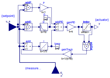
Via parameter controllerType either P, PI, PD, or PID can be selected. If, e.g., PI is selected, all components belonging to the D-part are removed from the block (via conditional declarations). The example model Modelica.Blocks.Examples.PID_Controller demonstrates the usage of this controller. Several practical aspects of PID controller design are incorporated according to chapter 3 of the book:
Besides the additive proportional, integral and derivative part of this controller, the following features are present:
The parameters of the controller can be manually adjusted by performing simulations of the closed loop system (= controller + plant connected together) and using the following strategy:
Initialization
This block can be initialized in different ways controlled by parameter initType. The possible values of initType are defined in Modelica.Blocks.Types.InitPID. This type is identical to Types.Init, with the only exception that the additional option DoNotUse_InitialIntegratorState is added for backward compatibility reasons (= integrator is initialized with InitialState whereas differential part is initialized with NoInit which was the initialization in version 2.2 of the Modelica standard library).
Based on the setting of initType, the integrator (I) and derivative (D) blocks inside the PID controller are initialized according to the following table:
| initType | I.initType | D.initType |
| NoInit | NoInit | NoInit |
| SteadyState | SteadyState | SteadyState |
| InitialState | InitialState | InitialState |
| InitialOutput and initial equation: y = y_start |
NoInit | SteadyState |
| DoNotUse_InitialIntegratorState | InitialState | NoInit |
In many cases, the most useful initial condition is SteadyState because initial transients are then no longer present. If initType = InitPID.SteadyState, then in some cases difficulties might occur. The reason is the equation of the integrator:
der(y) = k*u;
The steady state equation "der(x)=0" leads to the condition that the input u to the integrator is zero. If the input u is already (directly or indirectly) defined by another initial condition, then the initialization problem is singular (has none or infinitely many solutions). This situation occurs often for mechanical systems, where, e.g., u = desiredSpeed - measuredSpeed and since speed is both a state and a derivative, it is natural to initialize it with zero. As sketched this is, however, not possible. The solution is to not initialize u_m or the variable that is used to compute u_m by an algebraic equation.
If parameter limitAtInit = false, the limits at the output of this controller block are removed from the initialization problem which leads to a much simpler equation system. After initialization has been performed, it is checked via an assert whether the output is in the defined limits. For backward compatibility reasons limitAtInit = true. In most cases it is best to use limitAtInit = false.
Extends from Interfaces.SVcontrol (Single-Variable continuous controller).
| Type | Name | Default | Description |
|---|---|---|---|
| SimpleController | controllerType | Modelica.Blocks.Types.Simple... | Type of controller |
| Real | k | 1 | Gain of controller [1] |
| Time | Ti | Time constant of Integrator block [s] | |
| Time | Td | Time constant of Derivative block [s] | |
| Real | yMax | Upper limit of output | |
| Real | yMin | -yMax | Lower limit of output |
| Real | wp | 1 | Set-point weight for Proportional block (0..1) |
| Real | wd | 0 | Set-point weight for Derivative block (0..1) |
| Real | Ni | 0.9 | Ni*Ti is time constant of anti-windup compensation |
| Real | Nd | 10 | The higher Nd, the more ideal the derivative block |
| Initialization | |||
| InitPID | initType | Modelica.Blocks.Types.InitPI... | Type of initialization (1: no init, 2: steady state, 3: initial state, 4: initial output) |
| Boolean | limitsAtInit | true | = false, if limits are ignored during initializiation |
| Real | xi_start | 0 | Initial or guess value value for integrator output (= integrator state) |
| Real | xd_start | 0 | Initial or guess value for state of derivative block |
| Real | y_start | 0 | Initial value of output |
| Type | Name | Description |
|---|---|---|
| input RealInput | u_s | Connector of setpoint input signal |
| input RealInput | u_m | Connector of measurement input signal |
| output RealOutput | y | Connector of actuator output signal |
block LimPID
  "P, PI, PD, and PID controller with limited output, anti-windup compensation and setpoint weighting"
  import Modelica.Blocks.Types.InitPID;
  import Modelica.Blocks.Types.SimpleController;
  extends Interfaces.SVcontrol;
  output Real controlError = u_s - u_m
    "Control error (set point - measurement)";

  parameter Modelica.Blocks.Types.SimpleController controllerType=
         Modelica.Blocks.Types.SimpleController.PID "Type of controller";
  parameter Real k(min=0, unit="1") = 1 "Gain of controller";
  parameter SIunits.Time Ti(min=Modelica.Constants.small, start=0.5)
    "Time constant of Integrator block";
  parameter SIunits.Time Td(min=0, start= 0.1)
    "Time constant of Derivative block";
  parameter Real yMax(start=1) "Upper limit of output";
  parameter Real yMin=-yMax "Lower limit of output";
  parameter Real wp(min=0) = 1 "Set-point weight for Proportional block (0..1)";
  parameter Real wd(min=0) = 0 "Set-point weight for Derivative block (0..1)";
  parameter Real Ni(min=100*Modelica.Constants.eps) = 0.9
    "Ni*Ti is time constant of anti-windup compensation";
  parameter Real Nd(min=100*Modelica.Constants.eps) = 10
    "The higher Nd, the more ideal the derivative block";
  parameter Modelica.Blocks.Types.InitPID initType= Modelica.Blocks.Types.InitPID.DoNotUse_InitialIntegratorState
    "Type of initialization (1: no init, 2: steady state, 3: initial state, 4: initial output)";
  parameter Boolean limitsAtInit = true
    "= false, if limits are ignored during initializiation";
  parameter Real xi_start=0
    "Initial or guess value value for integrator output (= integrator state)";
  parameter Real xd_start=0
    "Initial or guess value for state of derivative block";
  parameter Real y_start=0 "Initial value of output";

  Blocks.Math.Add addP(k1=wp, k2=-1);
  Blocks.Math.Add addD(k1=wd, k2=-1) if with_D;
  Blocks.Math.Gain P(k=1);
  Blocks.Continuous.Integrator I(k=1/Ti, y_start=xi_start,
    initType=if initType==InitPID.SteadyState then
                InitPID.SteadyState else
             if initType==InitPID.InitialState or
                initType==InitPID.DoNotUse_InitialIntegratorState then
                InitPID.InitialState else InitPID.NoInit) if with_I;
  Blocks.Continuous.Derivative D(k=Td, T=max([Td/Nd, 1.e-14]), x_start=xd_start,
    initType=if initType==InitPID.SteadyState or
                initType==InitPID.InitialOutput then InitPID.SteadyState else
             if initType==InitPID.InitialState then InitPID.InitialState else
                InitPID.NoInit) if with_D;
  Blocks.Math.Gain gainPID(k=k);
  Blocks.Math.Add3 addPID;
  Blocks.Math.Add3 addI(k2=-1) if with_I;
  Blocks.Math.Add addSat(k1=+1, k2=-1) if
                                   with_I;
  Blocks.Math.Gain gainTrack(k=1/(k*Ni)) if with_I;
  Blocks.Nonlinear.Limiter limiter(uMax=yMax, uMin=yMin, limitsAtInit=limitsAtInit);
protected
  parameter Boolean with_I = controllerType==SimpleController.PI or
                             controllerType==SimpleController.PID;
  parameter Boolean with_D = controllerType==SimpleController.PD or
                             controllerType==SimpleController.PID;
public
  Sources.Constant Dzero(k=0) if not with_D;
  Sources.Constant Izero(k=0) if not with_I;
initial equation
  if initType==InitPID.InitialOutput then
     y = y_start;
  end if;
equation
  assert(yMax >= yMin, "LimPID: Limits must be consistent. However, yMax (=" + String(yMax) +
                       ") < yMin (=" + String(yMin) + ")");
  if initType == InitPID.InitialOutput and (y_start < yMin or y_start > yMax) then
      Modelica.Utilities.Streams.error("LimPID: Start value y_start (=" + String(y_start) +
         ") is outside of the limits of yMin (=" + String(yMin) +") and yMax (=" + String(yMax) + ")");
  end if;
  assert(limitsAtInit or not limitsAtInit and y >= yMin and y <= yMax,
         "LimPID: During initialization the limits have been switched off.\n" +
         "After initialization, the output y (=" + String(y) +
         ") is outside of the limits of yMin (=" + String(yMin) +") and yMax (=" + String(yMax) + ")");

  connect(u_s, addP.u1);
  connect(u_s, addD.u1);
  connect(u_s, addI.u1);
  connect(addP.y, P.u);
  connect(addD.y, D.u);
  connect(addI.y, I.u);
  connect(P.y, addPID.u1);
  connect(D.y, addPID.u2);
  connect(I.y, addPID.u3);
  connect(addPID.y, gainPID.u);
  connect(gainPID.y, addSat.u2);
  connect(gainPID.y, limiter.u);
  connect(limiter.y, addSat.u1);
  connect(limiter.y, y);
  connect(addSat.y, gainTrack.u);
  connect(gainTrack.y, addI.u3);
  connect(u_m, addP.u2);
  connect(u_m, addD.u2);
  connect(u_m, addI.u2);
  connect(Dzero.y, addPID.u2);
  connect(Izero.y, addPID.u3);
end LimPID;
 Modelica.Blocks.Continuous.TransferFunction
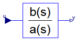
This block defines the transfer function between the input u and the output y as (nb = dimension of b, na = dimension of a):
           b[1]*s^[nb-1] + b[2]*s^[nb-2] + ... + b[nb]
   y(s) = --------------------------------------------- * u(s)
           a[1]*s^[na-1] + a[2]*s^[na-2] + ... + a[na]
State variables x are defined according to controller canonical form. Internally, vector x is scaled to improve the numerics (the states in versions before version 3.0 of the Modelica Standard Library have been not scaled). This scaling is not visible from the outside of this block because the non-scaled vector x is provided as output signal and the start value is with respect to the non-scaled vector x. Initial values of the states x can be set via parameter x_start.
Example:
TransferFunction g(b = {2,4}, a = {1,3});
results in the following transfer function:
        2*s + 4
   y = --------- * u
         s + 3
Extends from Interfaces.SISO (Single Input Single Output continuous control block).
| Type | Name | Default | Description |
|---|---|---|---|
| Real | b[:] | {1} | Numerator coefficients of transfer function (e.g., 2*s+3 is specified as {2,3}) |
| Real | a[:] | {1} | Denominator coefficients of transfer function (e.g., 5*s+6 is specified as {5,6}) |
| Initialization | |||
| Init | initType | Modelica.Blocks.Types.Init.N... | Type of initialization (1: no init, 2: steady state, 3: initial state, 4: initial output) |
| Real | x_start[size(a, 1) - 1] | zeros(nx) | Initial or guess values of states |
| Real | y_start | 0 | Initial value of output (derivatives of y are zero upto nx-1-th derivative) |
| Type | Name | Description |
|---|---|---|
| input RealInput | u | Connector of Real input signal |
| output RealOutput | y | Connector of Real output signal |
block TransferFunction "Linear transfer function"
  import Modelica.Blocks.Types.Init;
  extends Interfaces.SISO;

  parameter Real b[:]={1}
    "Numerator coefficients of transfer function (e.g., 2*s+3 is specified as {2,3})";
  parameter Real a[:]={1}
    "Denominator coefficients of transfer function (e.g., 5*s+6 is specified as {5,6})";
  parameter Modelica.Blocks.Types.Init initType=Modelica.Blocks.Types.Init.NoInit
    "Type of initialization (1: no init, 2: steady state, 3: initial state, 4: initial output)";
  parameter Real x_start[size(a, 1) - 1]=zeros(nx)
    "Initial or guess values of states";
  parameter Real y_start=0
    "Initial value of output (derivatives of y are zero upto nx-1-th derivative)";
  output Real x[size(a, 1) - 1](start=x_start)
    "State of transfer function from controller canonical form";
protected
  parameter Integer na=size(a, 1) "Size of Denominator of transfer function.";
  parameter Integer nb=size(b, 1) "Size of Numerator of transfer function.";
  parameter Integer nx=size(a, 1) - 1;
  parameter Real bb[:] = vector([zeros(max(0,na-nb),1);b]);
  parameter Real d = bb[1]/a[1];
  parameter Real a_end = if a[end] > 100*Modelica.Constants.eps*sqrt(a*a) then a[end] else 1.0;
  Real x_scaled[size(x,1)] "Scaled vector x";

initial equation
  if initType == Init.SteadyState then
    der(x_scaled) = zeros(nx);
  elseif initType == Init.InitialState then
    x_scaled = x_start*a_end;
  elseif initType == Init.InitialOutput then
    y = y_start;
    der(x_scaled[2:nx]) = zeros(nx-1);
  end if;
equation
  assert(size(b,1) <= size(a,1), "Transfer function is not proper");
  if nx == 0 then
     y = d*u;
  else
     der(x_scaled[1])    = (-a[2:na]*x_scaled + a_end*u)/a[1];
     der(x_scaled[2:nx]) = x_scaled[1:nx-1];
     y = ((bb[2:na] - d*a[2:na])*x_scaled)/a_end + d*u;
     x = x_scaled/a_end;
  end if;
end TransferFunction;
 Modelica.Blocks.Continuous.StateSpace
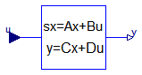
The State Space block defines the relation between the input u and the output y in state space form:
    der(x) = A * x + B * u
        y  = C * x + D * u
The input is a vector of length nu, the output is a vector of length ny and nx is the number of states. Accordingly
        A has the dimension: A(nx,nx),
        B has the dimension: B(nx,nu),
        C has the dimension: C(ny,nx),
        D has the dimension: D(ny,nu)
Example:
     parameter: A = [0.12, 2;3, 1.5]
     parameter: B = [2, 7;3, 1]
     parameter: C = [0.1, 2]
     parameter: D = zeros(ny,nu)
results in the following equations:
  [der(x[1])]   [0.12  2.00] [x[1]]   [2.0  7.0] [u[1]]
  [         ] = [          ]*[    ] + [        ]*[    ]
  [der(x[2])]   [3.00  1.50] [x[2]]   [0.1  2.0] [u[2]]
                             [x[1]]            [u[1]]
       y[1]   = [0.1  2.0] * [    ] + [0  0] * [    ]
                             [x[2]]            [u[2]]
Extends from Interfaces.MIMO (Multiple Input Multiple Output continuous control block).
| Type | Name | Default | Description |
|---|---|---|---|
| Real | A[:, size(A, 1)] | Matrix A of state space model (e.g., A=[1, 0; 0, 1]) | |
| Real | B[size(A, 1), :] | Matrix B of state space model (e.g., B=[1; 1]) | |
| Real | C[:, size(A, 1)] | Matrix C of state space model (e.g., C=[1, 1]) | |
| Real | D[size(C, 1), size(B, 2)] | zeros(size(C, 1), size(B, 2)) | Matrix D of state space model |
| Integer | nin | size(B, 2) | Number of inputs |
| Integer | nout | size(C, 1) | Number of outputs |
| Initialization | |||
| Init | initType | Modelica.Blocks.Types.Init.N... | Type of initialization (1: no init, 2: steady state, 3: initial state, 4: initial output) |
| Real | x_start[nx] | zeros(nx) | Initial or guess values of states |
| Real | y_start[ny] | zeros(ny) | Initial values of outputs (remaining states are in steady state if possible) |
| Type | Name | Description |
|---|---|---|
| input RealInput | u[nin] | Connector of Real input signals |
| output RealOutput | y[nout] | Connector of Real output signals |
block StateSpace "Linear state space system"
  import Modelica.Blocks.Types.Init;
  parameter Real A[:, size(A, 1)]
    "Matrix A of state space model (e.g., A=[1, 0; 0, 1])";
  parameter Real B[size(A, 1), :]
    "Matrix B of state space model (e.g., B=[1; 1])";
  parameter Real C[:, size(A, 1)]
    "Matrix C of state space model (e.g., C=[1, 1])";
  parameter Real D[size(C, 1), size(B, 2)]=zeros(size(C, 1), size(B, 2))
    "Matrix D of state space model";
  parameter Modelica.Blocks.Types.Init initType=Modelica.Blocks.Types.Init.NoInit
    "Type of initialization (1: no init, 2: steady state, 3: initial state, 4: initial output)";
  parameter Real x_start[nx]=zeros(nx) "Initial or guess values of states";
  parameter Real y_start[ny]=zeros(ny)
    "Initial values of outputs (remaining states are in steady state if possible)";

  extends Interfaces.MIMO(final nin=size(B, 2), final nout=size(C, 1));
  output Real x[size(A, 1)](start=x_start) "State vector";

protected
  parameter Integer nx = size(A, 1) "number of states";
  parameter Integer ny = size(C, 1) "number of outputs";
initial equation
  if initType == Init.SteadyState then
    der(x) = zeros(nx);
  elseif initType == Init.InitialState then
    x = x_start;
  elseif initType == Init.InitialOutput then
    x = Modelica.Math.Matrices.equalityLeastSquares(A, -B*u, C, y_start - D*u);
  end if;
equation
  der(x) = A*x + B*u;
  y = C*x + D*u;
end StateSpace;
 Modelica.Blocks.Continuous.Der

Defines that the output y is the derivative of the input u. Note, that Modelica.Blocks.Continuous.Derivative computes the derivative in an approximate sense, where as this block computes the derivative exactly. This requires that the input u is differentiated by the Modelica translator, if this derivative is not yet present in the model.
Extends from Interfaces.SISO (Single Input Single Output continuous control block).
| Type | Name | Description |
|---|---|---|
| input RealInput | u | Connector of Real input signal |
| output RealOutput | y | Connector of Real output signal |
block Der "Derivative of input (= analytic differentations)"
    extends Interfaces.SISO;

equation
  y = der(u);
end Der;
 Modelica.Blocks.Continuous.LowpassButterworth
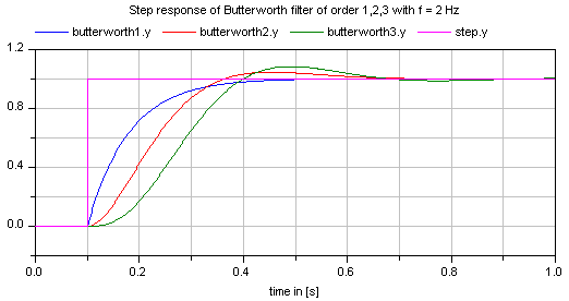
This block defines the transfer function between the input u and the output y as an n-th order low pass filter with Butterworth characteristics and cut-off frequency f. It is implemented as a series of second order filters and a first order filter. Butterworth filters have the feature that the amplitude at the cut-off frequency f is 1/sqrt(2) (= 3 dB), i.e., they are always "normalized". Step responses of the Butterworth filter of different orders are shown in the next figure:
If transients at the simulation start shall be avoided, the filter should be initialized in steady state (e.g., using option initType=Modelica.Blocks.Types.Init.SteadyState).
Extends from Modelica.Blocks.Interfaces.SISO (Single Input Single Output continuous control block).
| Type | Name | Default | Description |
|---|---|---|---|
| Integer | n | 2 | Order of filter |
| Frequency | f | Cut-off frequency [Hz] | |
| Initialization | |||
| Init | initType | Modelica.Blocks.Types.Init.N... | Type of initialization (1: no init, 2: steady state, 3: initial state, 4: initial output) |
| Real | x1_start[m] | zeros(m) | Initial or guess values of states 1 (der(x1)=x2)) |
| Real | x2_start[m] | zeros(m) | Initial or guess values of states 2 |
| Real | xr_start | 0.0 | Initial or guess value of real pole for uneven order otherwise dummy |
| Real | y_start | 0.0 | Initial value of output (states are initialized in steady state if possible) |
| Type | Name | Description |
|---|---|---|
| input RealInput | u | Connector of Real input signal |
| output RealOutput | y | Connector of Real output signal |
block LowpassButterworth
  "Output the input signal filtered with a low pass Butterworth filter of any order"

  import Modelica.Math.*;
  import Modelica.Blocks.Types.Init;

  extends Modelica.Blocks.Interfaces.SISO;

  parameter Integer n(min=1) = 2 "Order of filter";
  parameter SI.Frequency f(start=1) "Cut-off frequency";
  parameter Modelica.Blocks.Types.Init initType=Modelica.Blocks.Types.Init.NoInit
    "Type of initialization (1: no init, 2: steady state, 3: initial state, 4: initial output)";
  parameter Real x1_start[m]=zeros(m)
    "Initial or guess values of states 1 (der(x1)=x2))";
  parameter Real x2_start[m]=zeros(m) "Initial or guess values of states 2";
  parameter Real xr_start=0.0
    "Initial or guess value of real pole for uneven order otherwise dummy";
  parameter Real y_start=0.0
    "Initial value of output (states are initialized in steady state if possible)";

  output Real x1[m](start=x1_start)
    "states 1 of second order filters (der(x1) = x2)";
  output Real x2[m](start=x2_start) "states 2 of second order filters";
  output Real xr(start=xr_start)
    "state of real pole for uneven order otherwise dummy";
protected
  constant Real pi=Modelica.Constants.pi;
  parameter Integer m=integer(n/2);
  parameter Boolean evenOrder = 2*m == n;
  parameter Real w=2*pi*f;
  Real z[m + 1];
  Real polereal[m];
  Real poleimag[m];
  Real realpol;
  Real k2[m];
  Real D[m];
  Real w0[m];
  Real k1;
  Real T;
initial equation
  if initType == Init.SteadyState then
    der(x1) = zeros(m);
    der(x2) = zeros(m);
    if not evenOrder then
      der(xr) = 0.0;
    end if;
  elseif initType == Init.InitialState then
    x1 = x1_start;
    x2 = x2_start;
    if not evenOrder then
      xr = xr_start;
    end if;
  elseif initType == Init.InitialOutput then
    y = y_start;
    der(x1) = zeros(m);
    if evenOrder then
      if m > 1 then
        der(x2[1:m-1]) = zeros(m-1);
      end if;
    else
      der(x1) = zeros(m);
    end if;
  end if;
equation
  k2 = ones(m);
  k1 = 1;
  z[1] = u;

  // calculate filter parameters
  for i in 1:m loop
    // poles of prototype lowpass
    polereal[i] = cos(pi/2 + pi/n*(i - 0.5));
    poleimag[i] = sin(pi/2 + pi/n*(i - 0.5));
    // scaling and calculation of secon order filter coefficients
    w0[i] = (polereal[i]^2 + poleimag[i]^2)*w;
    D[i] = -polereal[i]/w0[i]*w;
  end for;
  realpol = 1*w;
  T = 1/realpol;

  // calculate second order filters
  for i in 1:m loop
    der(x1[i]) = x2[i];
    der(x2[i]) = k2[i]*w0[i]^2*z[i] - 2*D[i]*w0[i]*x2[i] - w0[i]^2*x1[i];
    z[i + 1] = x1[i];
  end for;

  // calculate first order filter if necessary
  if evenOrder then
    // even order
    xr = 0;
    y = z[m + 1];
  else
    // uneven order
    der(xr) = (k1*z[m + 1] - xr)/T;
    y = xr;
  end if;
end LowpassButterworth;
 Modelica.Blocks.Continuous.CriticalDamping
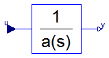
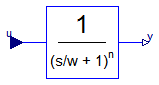
This block defines the transfer function between the input u and the output y as an n-th order filter with critical damping characteristics and cut-off frequency f. It is implemented as a series of first order filters. This filter type is especially useful to filter the input of an inverse model, since the filter does not introduce any transients.
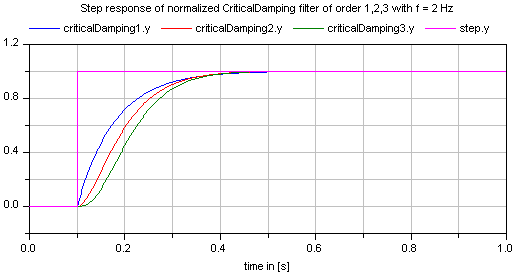
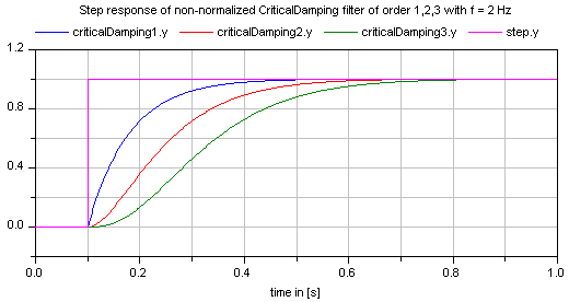
If parameter normalized = true (default), the filter is normalized such that the amplitude of the filter transfer function at the cut-off frequency f is 1/sqrt(2) (= 3 dB). Otherwise, the filter is not normalized, i.e., it is unmodified. A normalized filter is usually much better for applications, since filters of different orders are "comparable", whereas non-normalized filters usually require to adapt the cut-off frequency, when the order of the filter is changed. Figures of the filter step responses are shown below. Note, in versions before version 3.0 of the Modelica Standard library, the CriticalDamping filter was provided only in non-normalzed form.
If transients at the simulation start shall be avoided, the filter should be initialized in steady state (e.g., using option initType=Modelica.Blocks.Types.Init.SteadyState).
The critical damping filter is defined as
    α = if normalized then sqrt(2^(1/n) - 1) else 1 // frequency correction factor
    ω = 2*π*f/α
              1
    y = ------------- * u
         (s/w + 1)^n
Extends from Modelica.Blocks.Interfaces.SISO (Single Input Single Output continuous control block).
| Type | Name | Default | Description |
|---|---|---|---|
| Integer | n | 2 | Order of filter |
| Frequency | f | Cut-off frequency [Hz] | |
| Boolean | normalized | true | = true, if amplitude at f_cut is 3 dB, otherwise unmodified filter |
| Initialization | |||
| Init | initType | Modelica.Blocks.Types.Init.N... | Type of initialization (1: no init, 2: steady state, 3: initial state, 4: initial output) |
| Real | x_start[n] | zeros(n) | Initial or guess values of states |
| Real | y_start | 0.0 | Initial value of output (remaining states are in steady state) |
| Type | Name | Description |
|---|---|---|
| input RealInput | u | Connector of Real input signal |
| output RealOutput | y | Connector of Real output signal |
block CriticalDamping
  "Output the input signal filtered with an n-th order filter with critical damping"

  import Modelica.Blocks.Types.Init;
  extends Modelica.Blocks.Interfaces.SISO;

  parameter Integer n=2 "Order of filter";
  parameter Modelica.SIunits.Frequency f(start=1) "Cut-off frequency";
  parameter Boolean normalized = true
    "= true, if amplitude at f_cut is 3 dB, otherwise unmodified filter";
  parameter Modelica.Blocks.Types.Init initType=Modelica.Blocks.Types.Init.NoInit
    "Type of initialization (1: no init, 2: steady state, 3: initial state, 4: initial output)";
  parameter Real x_start[n]=zeros(n) "Initial or guess values of states";
  parameter Real y_start=0.0
    "Initial value of output (remaining states are in steady state)";

  output Real x[n](start=x_start) "Filter states";
protected
  parameter Real alpha=if normalized then sqrt(2^(1/n) - 1) else 1.0
    "Frequency correction factor for normalized filter";
  parameter Real w=2*Modelica.Constants.pi*f/alpha;
initial equation
  if initType == Init.SteadyState then
    der(x) = zeros(n);
  elseif initType == Init.InitialState then
    x = x_start;
  elseif initType == Init.InitialOutput then
    y = y_start;
    der(x[1:n-1]) = zeros(n-1);
  end if;
equation
  der(x[1]) = (u - x[1])*w;
  for i in 2:n loop
    der(x[i]) = (x[i - 1] - x[i])*w;
  end for;
  y = x[n];
end CriticalDamping;
 Modelica.Blocks.Continuous.Filter
This blocks models various types of filters:
low pass, high pass, band pass, and band stop filters
using various filter characteristics:
CriticalDamping, Bessel, Butterworth, Chebyshev Type I filters
By default, a filter block is initialized in steady-state, in order to avoid unwanted osciallations at the beginning. In special cases, it might be useful to select one of the other initialization options under tab "Advanced".
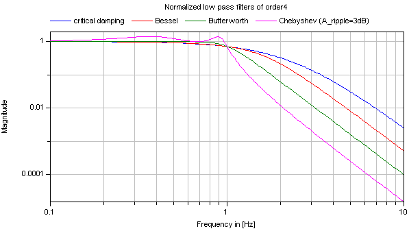
Typical frequency responses for the 4 supported low pass filter types are shown in the next figure:
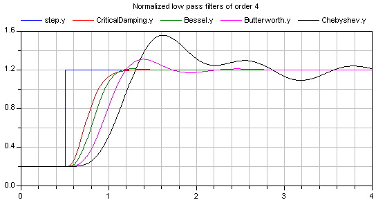
The step responses of the same low pass filters are shown in the next figure, starting from a steady state initial filter with initial input = 0.2:
Obviously, the frequency responses give a somewhat wrong impression of the filter characteristics: Although Butterworth and Chebyshev filters have a significantly steeper magnitude as the CriticalDamping and Bessel filters, the step responses of the latter ones are much better. This means for example, that a CriticalDamping or a Bessel filter should be selected, if a filter is mainly used to make a non-linear inverse model realizable.
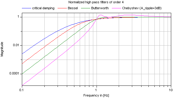
Typical frequency responses for the 4 supported high pass filter types are shown in the next figure:
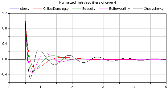
The corresponding step responses of these high pass filters are shown in the next figure:
All filters are available in normalized (default) and non-normalized form. In the normalized form, the amplitude of the filter transfer function at the cut-off frequency f_cut is -3 dB (= 10^(-3/20) = 0.70794..). Note, when comparing the filters of this function with other software systems, the setting of "normalized" has to be selected appropriately. For example, the signal processing toolbox of Matlab provides the filters in non-normalized form and therefore a comparision makes only sense, if normalized = false is set. A normalized filter is usually better suited for applications, since filters of different orders are "comparable", whereas non-normalized filters usually require to adapt the cut-off frequency, when the order of the filter is changed. See a comparision of "normalized" and "non-normalized" filters at hand of CriticalDamping filters of order 1,2,3:
The filters are implemented in the following, reliable way:
  // second order block with eigen values: a +/- jb
  der(x1) = a*x1 - b*x2 + (a^2 + b^2)/b*u;
  der(x2) = b*x1 + a*x2;
       y  = x2;
The dc-gain from the input to the output of this block is one and the selected
states are in the order of the input (if "u" is in the order of "one", then the
states are also in the order of "one"). In the "Advanced" tab, a "nominal" value for
the input "u" can be given. If appropriately selected, the states are in the order of "one" and
then step-size control is always appropriate.Extends from Modelica.Blocks.Interfaces.SISO (Single Input Single Output continuous control block).
| Type | Name | Default | Description |
|---|---|---|---|
| AnalogFilter | analogFilter | Modelica.Blocks.Types.Analog... | Analog filter characteristics (CriticalDamping/Bessel/Butterworth/ChebyshevI) |
| FilterType | filterType | Modelica.Blocks.Types.Filter... | Type of filter (LowPass/HighPass/BandPass/BandStop) |
| Integer | order | 2 | Order of filter |
| Frequency | f_cut | Cut-off frequency [Hz] | |
| Real | gain | 1.0 | Gain (= amplitude of frequency response at zero frequency) |
| Real | A_ripple | 0.5 | Pass band ripple for Chebyshev filter (otherwise not used); > 0 required [dB] |
| Frequency | f_min | 0 | Band of band pass/stop filter is f_min (A=-3db*gain) .. f_cut (A=-3db*gain) [Hz] |
| Boolean | normalized | true | = true, if amplitude at f_cut = -3db, otherwise unmodified filter |
| Advanced | |||
| Init | init | Modelica.Blocks.Types.Init.S... | Type of initialization (no init/steady state/initial state/initial output) |
| Real | x_start[nx] | zeros(nx) | Initial or guess values of states |
| Real | y_start | 0 | Initial value of output |
| Real | u_nominal | 1.0 | Nominal value of input (used for scaling the states) |
| Type | Name | Description |
|---|---|---|
| input RealInput | u | Connector of Real input signal |
| output RealOutput | y | Connector of Real output signal |
| output RealOutput | x[nx] | Filter states |
block Filter
  "Continuous low pass, high pass, band pass or band stop IIR-filter of type CriticalDamping, Bessel, Butterworth or ChebyshevI"
  import Modelica.Blocks.Continuous.Internal;

  extends Modelica.Blocks.Interfaces.SISO;

  parameter Modelica.Blocks.Types.AnalogFilter analogFilter=Modelica.Blocks.Types.AnalogFilter.CriticalDamping
    "Analog filter characteristics (CriticalDamping/Bessel/Butterworth/ChebyshevI)";
  parameter Modelica.Blocks.Types.FilterType filterType=Modelica.Blocks.Types.FilterType.LowPass
    "Type of filter (LowPass/HighPass/BandPass/BandStop)";
  parameter Integer order(min=1) = 2 "Order of filter";
  parameter Modelica.SIunits.Frequency f_cut "Cut-off frequency";
  parameter Real gain=1.0
    "Gain (= amplitude of frequency response at zero frequency)";
  parameter Real A_ripple(unit="dB") = 0.5
    "Pass band ripple for Chebyshev filter (otherwise not used); > 0 required";
  parameter Modelica.SIunits.Frequency f_min=0
    "Band of band pass/stop filter is f_min (A=-3db*gain) .. f_cut (A=-3db*gain)";
  parameter Boolean normalized=true
    "= true, if amplitude at f_cut = -3db, otherwise unmodified filter";
  parameter Modelica.Blocks.Types.Init init=Modelica.Blocks.Types.Init.SteadyState
    "Type of initialization (no init/steady state/initial state/initial output)";
  final parameter Integer nx = if filterType == Modelica.Blocks.Types.FilterType.LowPass or
                                  filterType == Modelica.Blocks.Types.FilterType.HighPass then
                                  order else 2*order;
  parameter Real x_start[nx] = zeros(nx) "Initial or guess values of states";
  parameter Real y_start = 0 "Initial value of output";
  parameter Real u_nominal = 1.0
    "Nominal value of input (used for scaling the states)";
  Modelica.Blocks.Interfaces.RealOutput x[nx] "Filter states";

protected
  parameter Integer ncr = if analogFilter == Modelica.Blocks.Types.AnalogFilter.CriticalDamping then
                             order else mod(order,2);
  parameter Integer nc0 = if analogFilter == Modelica.Blocks.Types.AnalogFilter.CriticalDamping then
                             0 else integer(order/2);
  parameter Integer na = if filterType == Modelica.Blocks.Types.FilterType.BandPass or
                            filterType == Modelica.Blocks.Types.FilterType.BandStop then order else
                         if analogFilter == Modelica.Blocks.Types.AnalogFilter.CriticalDamping then
                            0 else integer(order/2);
  parameter Integer nr = if filterType == Modelica.Blocks.Types.FilterType.BandPass or
                            filterType == Modelica.Blocks.Types.FilterType.BandStop then 0 else
                         if analogFilter == Modelica.Blocks.Types.AnalogFilter.CriticalDamping then
                            order else mod(order,2);

  // Coefficients of prototype base filter (low pass filter with w_cut = 1 rad/s)
  parameter Real cr[ncr](each fixed=false);
  parameter Real c0[nc0](each fixed=false);
  parameter Real c1[nc0](each fixed=false);

  // Coefficients for differential equations.
  parameter Real r[nr](each fixed=false);
  parameter Real a[na](each fixed=false);
  parameter Real b[na](each fixed=false);
  parameter Real ku[na](each fixed=false);
  parameter Real k1[if filterType == Modelica.Blocks.Types.FilterType.LowPass then 0 else na](
                 each fixed = false);
  parameter Real k2[if filterType == Modelica.Blocks.Types.FilterType.LowPass then 0 else na](
                 each fixed = false);

  // Auxiliary variables
  Real uu[na+nr+1];

initial equation
   if analogFilter == Modelica.Blocks.Types.AnalogFilter.CriticalDamping then
      cr = Internal.Filter.base.CriticalDamping(order, normalized);
   elseif analogFilter == Modelica.Blocks.Types.AnalogFilter.Bessel then
      (cr,c0,c1) = Internal.Filter.base.Bessel(order, normalized);
   elseif analogFilter == Modelica.Blocks.Types.AnalogFilter.Butterworth then
      (cr,c0,c1) = Internal.Filter.base.Butterworth(order, normalized);
   elseif analogFilter == Modelica.Blocks.Types.AnalogFilter.ChebyshevI then
      (cr,c0,c1) = Internal.Filter.base.ChebyshevI(order, A_ripple, normalized);
   end if;

   if filterType == Modelica.Blocks.Types.FilterType.LowPass then
      (r,a,b,ku) = Internal.Filter.roots.lowPass(cr,c0,c1,f_cut);
   elseif filterType == Modelica.Blocks.Types.FilterType.HighPass then
      (r,a,b,ku,k1,k2) = Internal.Filter.roots.highPass(cr,c0,c1,f_cut);
   elseif filterType == Modelica.Blocks.Types.FilterType.BandPass then
      (a,b,ku,k1,k2) = Internal.Filter.roots.bandPass(cr,c0,c1,f_min,f_cut);
   elseif filterType == Modelica.Blocks.Types.FilterType.BandStop then
      (a,b,ku,k1,k2) = Internal.Filter.roots.bandStop(cr,c0,c1,f_min,f_cut);
   end if;

   if init == Modelica.Blocks.Types.Init.InitialState then
      x = x_start;
   elseif init == Modelica.Blocks.Types.Init.SteadyState then
      der(x) = zeros(nx);
   elseif init == Modelica.Blocks.Types.Init.InitialOutput then
      y = y_start;
      if nx > 1 then
         der(x[1:nx-1]) = zeros(nx-1);
      end if;
   end if;

equation
   assert(u_nominal > 0, "u_nominal > 0 required");
   assert(filterType == Modelica.Blocks.Types.FilterType.LowPass or
          filterType == Modelica.Blocks.Types.FilterType.HighPass or
          f_min > 0, "f_min > 0 required for band pass and band stop filter");
   assert(A_ripple > 0, "A_ripple > 0 required");
   assert(f_cut > 0, "f_cut > 0  required");

   /* All filters have the same basic differential equations:
        Real poles:
           der(x) = r*x - r*u
        Complex conjugate poles:
           der(x1) = a*x1 - b*x2 + ku*u;
           der(x2) = b*x1 + a*x2;
   */
   uu[1] = u/u_nominal;
   for i in 1:nr loop
      der(x[i]) = r[i]*(x[i] - uu[i]);
   end for;
   for i in 1:na loop
      der(x[nr+2*i-1]) = a[i]*x[nr+2*i-1] - b[i]*x[nr+2*i] + ku[i]*uu[nr+i];
      der(x[nr+2*i])   = b[i]*x[nr+2*i-1] + a[i]*x[nr+2*i];
   end for;

   // The output equation is different for the different filter types
   if filterType == Modelica.Blocks.Types.FilterType.LowPass then
      /* Low pass filter
           Real poles             :  y = x
           Complex conjugate poles:  y = x2
      */
      for i in 1:nr loop
         uu[i+1] = x[i];
      end for;
      for i in 1:na loop
         uu[nr+i+1] = x[nr+2*i];
      end for;

   elseif filterType == Modelica.Blocks.Types.FilterType.HighPass then
      /* High pass filter
           Real poles             :  y = -x + u;
           Complex conjugate poles:  y = k1*x1 + k2*x2 + u;
      */
      for i in 1:nr loop
         uu[i+1] = -x[i] + uu[i];
      end for;
      for i in 1:na loop
         uu[nr+i+1] = k1[i]*x[nr+2*i-1] + k2[i]*x[nr+2*i] + uu[nr+i];
      end for;

   elseif filterType == Modelica.Blocks.Types.FilterType.BandPass then
      /* Band pass filter
           Complex conjugate poles:  y = k1*x1 + k2*x2;
      */
      for i in 1:na loop
         uu[nr+i+1] = k1[i]*x[nr+2*i-1] + k2[i]*x[nr+2*i];
      end for;

   elseif filterType == Modelica.Blocks.Types.FilterType.BandStop then
      /* Band pass filter
           Complex conjugate poles:  y = k1*x1 + k2*x2 + u;
      */
      for i in 1:na loop
         uu[nr+i+1] = k1[i]*x[nr+2*i-1] + k2[i]*x[nr+2*i] + uu[nr+i];
      end for;

   else
      assert(false, "filterType (= " + String(filterType) + ") is unknown");
      uu = zeros(na+nr+1);
   end if;

   y = (gain*u_nominal)*uu[nr+na+1];

end Filter;