Buildings.Controls.OBC.CDL.Continuous.Sources
Package with blocks that generate source signals
Information
Package with blocks that generate signals.
Package Content
| Name | Description |
|---|---|
| Computes the unix time stamp and calendar time from the simulation time | |
| Output constant signal of type Real | |
| Standard time | |
| Generate pulse signal of type Real | |
| Generate ramp signal | |
| Generate sine signal | |
| Table look-up with respect to time and linear or periodic extrapolation | |
| Collection of models that validate the continuous sources blocks of the CDL |
 Buildings.Controls.OBC.CDL.Continuous.Sources.CalendarTime
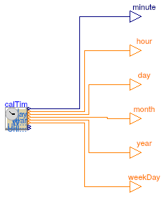
Computes the unix time stamp and calendar time from the simulation time
Information
Block that outputs minute, hour, day of the month, month, year and weekday.
Assumption and limitations
The implementation only supports date computations from year 2010 up to and including 2020. Daylight saving and time zones are not supported.
Typical use and important parameters
The user must define which time and date correspond to time = 0
using the model parameters zerTim, and, if
zerTim == CDL.Types.ZeroTime.Custom,
the parameter yearRef.
The user can choose from new year, midnight for a number of years:
2010 to 2020 and also 1970.
The latter corresponds to a unix stamp of 0.
Note that when choosing the reference time equal to 0 at 1970,
the actual simulation time must be within the 2010-2020 range.
For example, startTime = 1262304000 corresponds
to the simulation starting on the 1st of January 2010 local time
when setting zerTim = CDL.Types.ZeroTime.UnixTimeStamp.
This is within the 2010-2020 range and is therefore allowed.
Parameters
| Type | Name | Default | Description |
|---|---|---|---|
| ZeroTime | zerTim | Enumeration for choosing how reference time (time = 0) should be defined | |
| Integer | yearRef | 2016 | Year when time = 0, used if zerTim=Custom |
| Advanced | |||
| Time | offset | 0 | Offset that is added to 'time', may be used for computing time in different time zone [s] |
Connectors
| Type | Name | Description |
|---|---|---|
| output IntegerOutput | year | Year |
| output IntegerOutput | month | Month of the year |
| output IntegerOutput | day | Day of the month |
| output IntegerOutput | hour | Hour of the day |
| output RealOutput | minute | Minute of the hour |
| output IntegerOutput | weekDay | Integer output representing week day (monday = 1, sunday = 7) |
Modelica definition
 Buildings.Controls.OBC.CDL.Continuous.Sources.Constant
Output constant signal of type Real

Information
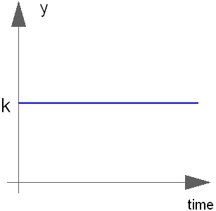
Block that outputs a constant signal y = k,
where k is a real-valued parameter.
Parameters
| Type | Name | Default | Description |
|---|---|---|---|
| Real | k | Constant output value |
Connectors
| Type | Name | Description |
|---|---|---|
| output RealOutput | y | Connector of Real output signal |
Modelica definition
 Buildings.Controls.OBC.CDL.Continuous.Sources.ModelTime
Standard time

Information
Block that outputs the standard time.
Implementation
This block outputs the time of the model. In the case of a building automation system, the building automation system synchronizes time, and hence need to assign a value for the output of this block. Daylight saving time shall not be taken into account, e.g, the block always outputs standard time rather than daylight savings time.
If a simulation starts at t=-1, then this block outputs first t=-1, and its output is advanced at the same rate as the simulation time.
Connectors
| Type | Name | Description |
|---|---|---|
| output RealOutput | y | Connector of Real output signal [s] |
Modelica definition
 Buildings.Controls.OBC.CDL.Continuous.Sources.Pulse
Generate pulse signal of type Real

Information
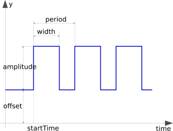
The Real output y is a pulse signal:
Parameters
| Type | Name | Default | Description |
|---|---|---|---|
| Real | amplitude | 1 | Amplitude of pulse |
| Real | width | 0.5 | Width of pulse in fraction of period [1] |
| Time | period | period(final min=Constants.s... | Time for one period [s] |
| Integer | nperiod | -1 | Number of periods (< 0 means infinite number of periods) |
| Real | offset | 0 | Offset of output signals |
| Time | startTime | 0 | Output = offset for time < startTime [s] |
Connectors
| Type | Name | Description |
|---|---|---|
| output RealOutput | y | Connector of Pulse output signal |
Modelica definition
 Buildings.Controls.OBC.CDL.Continuous.Sources.Ramp
Generate ramp signal

Information
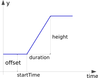
The Real output y is a ramp signal:
Parameters
| Type | Name | Default | Description |
|---|---|---|---|
| Real | height | 1 | Height of ramps |
| Time | duration | duration(min=Constants.small) | Duration of ramp (= 0.0 gives a Step) [s] |
| Real | offset | 0 | Offset of output signal |
| Time | startTime | 0 | Output = offset for time < startTime [s] |
Connectors
| Type | Name | Description |
|---|---|---|
| output RealOutput | y | Connector of Real output signal |
Modelica definition
 Buildings.Controls.OBC.CDL.Continuous.Sources.Sine
Generate sine signal

Information
Block that outputs a sine.
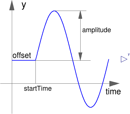
Parameters
| Type | Name | Default | Description |
|---|---|---|---|
| Real | amplitude | 1 | Amplitude of sine wave |
| Frequency | freqHz | freqHz(start=1) | Frequency of sine wave [Hz] |
| Angle | phase | 0 | Phase of sine wave [rad] |
| Real | offset | 0 | Offset of output signal |
| Time | startTime | 0 | Output = offset for time < startTime [s] |
Connectors
| Type | Name | Description |
|---|---|---|
| output RealOutput | y | Connector of Real output signal |
Modelica definition
 Buildings.Controls.OBC.CDL.Continuous.Sources.TimeTable
Table look-up with respect to time and linear or periodic extrapolation

Information
Block that outputs values of a time table.
The block takes as a parameter a time table of the format
table = [ 0*3600, 0;
          6*3600, 0;
          6*3600, 1;
         18*3600, 1;
         18*3600, 0;
         24*3600, 0];
where the first column is time in seconds, and the remaining
column(s) are the table values.
Any number of columns can be specified.
The parameter smoothness determines how the table values
are interpolated. The following settings are allowed:
smoothness | Description |
|---|---|
CDL.Types.LinearSegments |
Table points are linearly interpolated. |
CDL.Types.ConstantSegments |
Table points are not interpolated, but the previous tabulated value is returned. |
The parameter extrapolation determines how the table
values are extrapolated. The following settings are allowed:
extrapolation | Description |
|---|---|
CDL.Types.HoldLastPoint |
Hold the first or last table point outside of the table scope. |
CDL.Types.LastTwoPoints |
Extrapolate by using the derivative at the first or last table points outside of the table scope. |
CDL.Types.Periodic |
Repeat the table scope periodically with periodicity
(max(table[:, 1]-min(table[:, 1]))*timeScale). |
If extrapolation === CDL.Types.Periodic, then the above example
would give a schedule with periodicity of one day. The simulation can start at any time,
whether it is a multiple of a day or not, and positive or negative.
The value of the parameter offset is added to the tabulated
values.
The parameters timeScale is used to scale the first column
of the table. For example, set timeScale = 3600 if the first
column is in hour (because in CDL, the time unit is seconds).
If the table has only one row, no interpolation is performed and the table values of this row are just returned.
An interval boundary is defined by two identical time values following each other. For example
   table = [0, 0;
            1, 0;
            1, 1;
            2, 3;
            3, 5;
            3, 2;
            4, 4;
            5, 5];
defines three intervalls: 0..1, 1..3, 3..5. Within an interval the defined
interpolation method is applied (so the table outputs within an interval are
continuous if smoothness = CDL.Types.LinearSegments).
Example:
  table = [0, 0;
           1, 0;
           1, 1;
           2, 4;
           3, 9;
           4, 16];
  smoothness = CDL.Types.LinearSegments;

If, e.g., time = 1.0, the output y =  0.0 (before event), 1.0 (after event)
    e.g., time = 1.5, the output y =  2.5,
    e.g., time = 2.0, the output y =  4.0,
    e.g., time = 5.0, the output y = 23.0 (i.e., extrapolation via last 2 points).
Implementation
For simulation, no time events are generated within an interval in order that also intervals with many points do not reduce the simulation efficiency. If the table points are largely changing, it is adviseable to force time events by duplicating every time point (especially, if the model in which the table is present allows the variable step integrator to make large integrator steps). For example, if a sawtooth signal is defined with the table, it is more reliable to define the table as:
   table = [0, 0;
            1, 2;
            1, 2;
            2, 0;
            2, 0;
            3, 2;
            3, 2];
instead of
   table = [0, 0;
            1, 2;
            2, 0;
            3, 2];
because time events are then generated at every time point.
Building automation systems typically have discrete time semantics with fixed sampling times, and no notion of superdense time (in which a tabulated value can change without advancing time). Therefore, to implement a table with two equal time stamps, a CDL translator may parameterize a table in the building automation in such a way that the step change happens at the time indicated in the first column, whereas previous sampling times output the tabulated value at the last transition. For example,
table = [0, 0;
         1, 0;
         1, 1];
smoothness = CDL.Types.ConstantSegments;
may be converted such that a building automation system with a sampling time of 0.5 seconds outputs
  t = 0, 0.5, 1, ...
  y = 0, 0  , 1, ...
Parameters
| Type | Name | Default | Description |
|---|---|---|---|
| Real | table[:, :] | Table matrix (time = first column is time in seconds, unless timeScale <> 1) | |
| Smoothness | smoothness | CDL.Types.Smoothness.LinearS... | Smoothness of table interpolation |
| Extrapolation | extrapolation | CDL.Types.Extrapolation.Peri... | Extrapolation of data outside the definition range |
| Real | offset[:] | {0} | Offsets of output signals |
| Time | timeScale | 1 | Time scale of first table column. Set to 3600 if time in table is in hours [s] |
Connectors
| Type | Name | Description |
|---|---|---|
| output RealOutput | y[nout] | Output of the table |
