Buildings.Utilities.Math.Functions.Examples

Collection of models that illustrate model use and test models

Information

This package contains examples for the use of models that can be found in Buildings.Utilities.Math.Functions.

Extends from Modelica.Icons.ExamplesPackage (Icon for packages containing runnable examples).

Package Content

Name	Description
$Buildings.Utilities.Math.Functions.Examples.CubicHermite$ CubicHermite	Test problem for cubic hermite splines
$Buildings.Utilities.Math.Functions.Examples.InverseXDerivativeCheck$ InverseXDerivativeCheck	Model that checks the correct implementation of the 1st order derivative of InverseXRegularized
$Buildings.Utilities.Math.Functions.Examples.InverseXDerivative_2_Check$ InverseXDerivative_2_Check	Model that checks the correct implementation of the 2nd order derivative of InverseXRegularized
$Buildings.Utilities.Math.Functions.Examples.InverseXRegularized$ InverseXRegularized	Test problem for function that replaces 1/x around the origin by a twice continuously differentiable function
$Buildings.Utilities.Math.Functions.Examples.IsMonotonic$ IsMonotonic	Tests the correct implementation of the function isMonotonic
$Buildings.Utilities.Math.Functions.Examples.Polynomial$ Polynomial
$Buildings.Utilities.Math.Functions.Examples.PowerLinearized$ PowerLinearized	Test problem for function that linearizes y=x^n below some threshold
$Buildings.Utilities.Math.Functions.Examples.QuinticHermite$ QuinticHermite	Example model using quintic Hermite spline
$Buildings.Utilities.Math.Functions.Examples.RegNonZeroPower$ RegNonZeroPower
$Buildings.Utilities.Math.Functions.Examples.RegNonZeroPowerDerivativeCheck$ RegNonZeroPowerDerivativeCheck
$Buildings.Utilities.Math.Functions.Examples.RegNonZeroPowerDerivative_2_Check$ RegNonZeroPowerDerivative_2_Check
$Buildings.Utilities.Math.Functions.Examples.RegStep$ RegStep	Example for inlined regStep function
$Buildings.Utilities.Math.Functions.Examples.SmoothExponentialDerivativeCheck$ SmoothExponentialDerivativeCheck
$Buildings.Utilities.Math.Functions.Examples.SmoothInterpolation$ SmoothInterpolation	Test problem for cubic hermite splines that takes a vector of values as an argument
$Buildings.Utilities.Math.Functions.Examples.SpliceFunction$ SpliceFunction
$Buildings.Utilities.Math.Functions.Examples.SpliceFunctionDerivativeCheck$ SpliceFunctionDerivativeCheck
$Buildings.Utilities.Math.Functions.Examples.TrapezoidalIntegration$ TrapezoidalIntegration	Tests the correct implementation of the function trapezoidalIntegration

$Buildings.Utilities.Math.Functions.Examples.CubicHermite$ Buildings.Utilities.Math.Functions.Examples.CubicHermite

Test problem for cubic hermite splines

Information

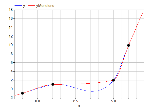
This example demonstrates the use of the function for cubic hermite interpolation and linear extrapolation. The example use interpolation with two different settings: One settings produces a monotone cubic hermite, whereas the other setting does not enforce monotonicity. The resulting plot should look as shown below, where for better visibility, the support points have been marked with black dots. Notice that the red curve is monotone increasing.

Extends from Modelica.Icons.Example (Icon for runnable examples).

Parameters

Type	Name	Default	Description
Real	xd[:]	{-1,1,5,6}	Support points
Real	yd[size(xd, 1)]	{-1,1,2,10}	Support points
Real	d[size(xd, 1)]		Derivatives at the support points
Real	dMonotone[size(xd, 1)]		Derivatives at the support points
Boolean	ensureMonotonicity	true

Modelica definition

model CubicHermite "Test problem for cubic hermite splines" extends Modelica.Icons.Example; parameter Real[:] xd={-1,1,5,6} "Support points"; parameter Real[size(xd, 1)] yd={-1,1,2,10} "Support points"; parameter Real[size(xd, 1)] d(each fixed=false) "Derivatives at the support points"; parameter Real[size(xd, 1)] dMonotone(each fixed=false) "Derivatives at the support points"; parameter Boolean ensureMonotonicity=true; Real x "Independent variable"; Real y "Dependent variable without monotone interpolation"; Real yMonotone "Dependent variable with monotone interpolation"; Integer i "Integer to select data interval"; initial algorithm // Get the derivative values at the support points d := Buildings.Utilities.Math.Functions.splineDerivatives( x=xd, y=yd, ensureMonotonicity=false); dMonotone := Buildings.Utilities.Math.Functions.splineDerivatives(x=xd, y=yd, ensureMonotonicity=true); algorithm x := xd[1] + time*1.2*(xd[size(xd, 1)] - xd[1]) - 0.5; // i is a counter that is used to pick the derivative of d or dMonotonic // that correspond to the interval that contains x i := 1; for j in 1:size(xd, 1) - 1 loop if x > xd[j] then i := j; end if; end for; // Extrapolate or interpolate the data y := Buildings.Utilities.Math.Functions.cubicHermiteLinearExtrapolation( x=x, x1=xd[i], x2=xd[i + 1], y1=yd[i], y2=yd[i + 1], y1d=d[i], y2d=d[i + 1]); yMonotone := Buildings.Utilities.Math.Functions.cubicHermiteLinearExtrapolation( x=x, x1=xd[i], x2=xd[i + 1], y1=yd[i], y2=yd[i + 1], y1d=dMonotone[i], y2d=dMonotone[i + 1]); end CubicHermite;

$Buildings.Utilities.Math.Functions.Examples.InverseXDerivativeCheck$ Buildings.Utilities.Math.Functions.Examples.InverseXDerivativeCheck

Model that checks the correct implementation of the 1st order derivative of InverseXRegularized

Information

This model validates the implementation of Buildings.Utilities.Math.Functions.inverseXRegularized and its first order derivative Buildings.Utilities.Math.Functions.BaseClasses.der_smoothTransition. If the derivative implementation is wrong, the simulation will stop with an error.

Extends from Modelica.Icons.Example (Icon for runnable examples).

Parameters

Type	Name	Default	Description
Real	delta	0.7	Smoothing coefficient

Modelica definition

model InverseXDerivativeCheck "Model that checks the correct implementation of the 1st order derivative of InverseXRegularized" extends Modelica.Icons.Example; constant Real gain = 4 "Gain for computing the mass flow rate"; parameter Real delta = 0.7 "Smoothing coefficient"; Real x "Independent variable"; Real y_comp "Comparison value"; Real y "Dependent variable"; Real err "Integration error"; initial equation y = y_comp; equation x = time^3*gain; y = Buildings.Utilities.Math.Functions.inverseXRegularized( x = x, delta = delta); der(y_comp) = Buildings.Utilities.Math.Functions.BaseClasses.der_inverseXRegularized(x=x,delta=delta,x_der=der(x)); err = y-y_comp; assert(abs(err) < 1E-3, "Error in implementation."); end InverseXDerivativeCheck;

$Buildings.Utilities.Math.Functions.Examples.InverseXDerivative_2_Check$ Buildings.Utilities.Math.Functions.Examples.InverseXDerivative_2_Check

Model that checks the correct implementation of the 2nd order derivative of InverseXRegularized

Information

This model validates the implementation of Buildings.Utilities.Math.Functions.inverseXRegularized and its second order derivative Buildings.Utilities.Math.Functions.BaseClasses.der_2_smoothTransition. If the derivative implementation is wrong, the simulation will stop with an error.

Extends from Modelica.Icons.Example (Icon for runnable examples).

Parameters

Type	Name	Default	Description
Real	delta	0.7	Smoothing coefficient

Modelica definition

model InverseXDerivative_2_Check "Model that checks the correct implementation of the 2nd order derivative of InverseXRegularized" extends Modelica.Icons.Example; Buildings.Utilities.Diagnostics.CheckEquality cheEqu1( threShold=1e-3) "Block for checking integration error"; Buildings.Utilities.Diagnostics.CheckEquality cheEqu2( threShold=1e-3) "Block for checking integration error"; constant Real gain = 4 "Gain for computing the mass flow rate"; parameter Real delta = 0.7 "Smoothing coefficient"; Real x "Independent variable"; Real y_comp "Comparison value"; Real y "Dependent variable"; Real der_y_comp "1st order derivative of comparison value"; Real der_y "1st order derivative of dependent variable"; Real err "Integration error"; Real der_err "Integration error"; initial equation y = y_comp; der_y = der_y_comp; equation x = time^3*gain; y = Buildings.Utilities.Math.Functions.inverseXRegularized( x = x, delta = delta); der_y = der(y); der_y_comp = der(y_comp); der(der_y) = der(der_y_comp); cheEqu1.u1 = y; cheEqu1.u2 = y_comp; err = cheEqu1.y; cheEqu2.u1 = der_y; cheEqu2.u2 = der_y_comp; der_err = cheEqu2.y; assert(abs(err) < 1E-3, "Error in implementation."); assert(abs(der_err) < 1E-3, "Error in implementation."); end InverseXDerivative_2_Check;

$Buildings.Utilities.Math.Functions.Examples.InverseXRegularized$ Buildings.Utilities.Math.Functions.Examples.InverseXRegularized

Test problem for function that replaces 1/x around the origin by a twice continuously differentiable function

Information

This example tests the implementation of Buildings.Utilities.Math.Functions.inverseXRegularized.

Extends from Modelica.Icons.Example (Icon for runnable examples).

Parameters

Type	Name	Default	Description
Real	delta	0.5	Small value for approximation

Modelica definition

model InverseXRegularized "Test problem for function that replaces 1/x around the origin by a twice continuously differentiable function" extends Modelica.Icons.Example; Real x "Independent variable"; parameter Real delta = 0.5 "Small value for approximation"; final parameter Real deltaInv = 1/delta "Inverse value of delta"; final parameter Real a = -15*deltaInv "Polynomial coefficient"; final parameter Real b = 119*deltaInv^2 "Polynomial coefficient"; final parameter Real c = -361*deltaInv^3 "Polynomial coefficient"; final parameter Real d = 534*deltaInv^4 "Polynomial coefficient"; final parameter Real e = -380*deltaInv^5 "Polynomial coefficient"; final parameter Real f = 104*deltaInv^6 "Polynomial coefficient"; Real y "Function value"; Real xInv "Function value"; Real dy_dt "First derivative of y with respect to t"; Real d2y_dt2 "Second derivative of y with respect to t"; equation x=2*time-1; xInv = if ( abs(x) > 0.1) then 1 / x else 0; y = Buildings.Utilities.Math.Functions.inverseXRegularized( x=x, delta=delta, deltaInv=deltaInv, a=a, b=b, c=c, d=d, e=e, f=f); dy_dt=der(y); d2y_dt2=der(dy_dt); end InverseXRegularized;

$Buildings.Utilities.Math.Functions.Examples.IsMonotonic$ Buildings.Utilities.Math.Functions.Examples.IsMonotonic

Tests the correct implementation of the function isMonotonic

Information

This example tests the correct implementation of the function Buildings.Utilities.Math.Functions.isMonotonic. If the function is implemented incorrect, the example will stop with an error.

Extends from Modelica.Icons.Example (Icon for runnable examples).

Modelica definition

model IsMonotonic "Tests the correct implementation of the function isMonotonic" extends Modelica.Icons.Example; Real x_incStrict[3] = {0, 1, 2} "strictly increasing"; Real x_notMon[3] = {0, 3, 2} "not monotonic"; Real x_incWeak[4] = {0, 1, 1, 2} "weakly increasing"; Real x_notWeak[4] = {0, 3, 3, 2} "not weakly monotonic"; Real x_decStrict[3] = {2.5, 2, 0.1} "strictly decreasing"; Real x_decWeak[4] = {3, 1, 1, 0.5} "weakly decreasing"; equation // Tests with weak monotonicity //strictly increasing assert(Buildings.Utilities.Math.Functions.isMonotonic(x_incStrict, strict=false), "Error. Function should have returned true."); //not monotonic assert(false == Buildings.Utilities.Math.Functions.isMonotonic(x_notMon, strict=false), "Error. Function should have returned true."); //weakly increasing assert(Buildings.Utilities.Math.Functions.isMonotonic(x_incWeak, strict=false), "Error. Function should have returned true."); //not weakly monotonic assert(false == Buildings.Utilities.Math.Functions.isMonotonic(x_notWeak, strict=false), "Error. Function should have returned true."); //strictly decreasing assert(Buildings.Utilities.Math.Functions.isMonotonic({2.5, 2, 0.1}, strict=false), "Error. Function should have returned true."); //weakly decreasing assert(Buildings.Utilities.Math.Functions.isMonotonic({3, 1, 1, 0.5}, strict=false), "Error. Function should have returned true."); // Tests with strict monotonicity //strictly increasing assert(Buildings.Utilities.Math.Functions.isMonotonic(x_incStrict, strict=true), "Error. Function should have returned true."); //not monotonic assert(false == Buildings.Utilities.Math.Functions.isMonotonic(x_notMon, strict=true), "Error. Function should have returned true."); //weakly increasing assert(false == Buildings.Utilities.Math.Functions.isMonotonic(x_incWeak, strict=true), "Error. Function should have returned true."); //not weakly monotonic assert(false == Buildings.Utilities.Math.Functions.isMonotonic(x_notWeak, strict=true), "Error. Function should have returned true."); //strictly decreasing assert(Buildings.Utilities.Math.Functions.isMonotonic(x_decStrict, strict=true), "Error. Function should have returned true."); //weakly decreasing assert(false == Buildings.Utilities.Math.Functions.isMonotonic(x_decWeak, strict=true), "Error. Function should have returned true."); end IsMonotonic;

$Buildings.Utilities.Math.Functions.Examples.Polynomial$ Buildings.Utilities.Math.Functions.Examples.Polynomial

Information

This example verifies the correct implementation of Buildings.Utilities.Math.Functions.polynomial.

Extends from Modelica.Icons.Example (Icon for runnable examples).

Modelica definition

model Polynomial extends Modelica.Icons.Example; Real x "Function value"; equation x=Buildings.Utilities.Math.Functions.polynomial(x=time^3-2, a={2, 4, -4, 5}); end Polynomial;

$Buildings.Utilities.Math.Functions.Examples.PowerLinearized$ Buildings.Utilities.Math.Functions.Examples.PowerLinearized

Test problem for function that linearizes y=x^n below some threshold

Information

This example tests the implementation of Buildings.Utilities.Math.Functions.powerLinearized.

Extends from Modelica.Icons.Example (Icon for runnable examples).

Modelica definition

model PowerLinearized "Test problem for function that linearizes y=x^n below some threshold" extends Modelica.Icons.Example; Real T4(start=300^4) "Temperature raised to 4-th power"; Real T "Temperature"; Real TExact "Temperature"; equation T = (1+500*time); T = Buildings.Utilities.Math.Functions.powerLinearized(x=T4, x0=243.15^4, n=0.25); TExact = abs(T4)^(1/4); end PowerLinearized;

$Buildings.Utilities.Math.Functions.Examples.QuinticHermite$ Buildings.Utilities.Math.Functions.Examples.QuinticHermite

Example model using quintic Hermite spline

Information

Demonstration of the use of a quintic Hermite spline interpolation function.

Extends from Modelica.Icons.Example (Icon for runnable examples).

Parameters

Type	Name	Default	Description
Real	a	0.5	Exponential argument coefficient
Real	x1	1	Lower abscissa value
Real	x2	2.6	Upper abscissa value
Real	y1	-x1	Lower ordinate value
Real	y1d	-1	Lower derivative
Real	y2d	aexp(ax2)	Upper derivative
Real	y1dd	0	Lower second derivative
Real	y2dd	a^2exp(ax2)	Upper second derivative

Modelica definition

model QuinticHermite "Example model using quintic Hermite spline" extends Modelica.Icons.Example; parameter Real a = 0.5 "Exponential argument coefficient"; parameter Real x1 = 1 "Lower abscissa value"; parameter Real x2 = 2.6 "Upper abscissa value"; parameter Real y1 = -x1 "Lower ordinate value"; parameter Real y1d = -1 "Lower derivative"; parameter Real y2d = a*exp(a*x2) "Upper derivative"; parameter Real y1dd = 0 "Lower second derivative"; parameter Real y2dd= a^2*exp(a*x2) "Upper second derivative"; Real x = time "Abscissa value"; Real y "Ordinate value"; Real dy "Time derivative of ordinate value"; Real ddy "Second time derivative of ordinate value"; Real y2 "Second ordinate section"; equation y2 = exp(a*x2); y= noEvent(smooth(2,if x>x2 then exp(a*x) elseif x<x1 then -time else Buildings.Utilities.Math.Functions.quinticHermite(x=x,x1=x1,x2=x2,y1=y1,y2=y2,y1d=y1d,y2d=y2d,y1dd=y1dd,y2dd=y2dd))); dy=der(y); ddy=der(dy); end QuinticHermite;

$Buildings.Utilities.Math.Functions.Examples.RegNonZeroPower$ Buildings.Utilities.Math.Functions.Examples.RegNonZeroPower

Information

This example tests the implementation of Buildings.Utilities.Math.Functions.regNonZeroPower.

Extends from Modelica.Icons.Example (Icon for runnable examples).

Modelica definition

model RegNonZeroPower extends Modelica.Icons.Example; Real y "Function value"; equation y=Buildings.Utilities.Math.Functions.regNonZeroPower( time, 0.3, 0.5); end RegNonZeroPower;

$Buildings.Utilities.Math.Functions.Examples.RegNonZeroPowerDerivativeCheck$ Buildings.Utilities.Math.Functions.Examples.RegNonZeroPowerDerivativeCheck

Information

This example checks whether the function derivative is implemented correctly. If the derivative implementation is not correct, the model will stop with an assert statement.

Extends from Modelica.Icons.Example (Icon for runnable examples).

Parameters

Type	Name	Default	Description
Real	n	0.33	Exponent
Real	delta	0.1	Abscissa value where transition occurs

Modelica definition

model RegNonZeroPowerDerivativeCheck extends Modelica.Icons.Example; parameter Real n=0.33 "Exponent"; parameter Real delta = 0.1 "Abscissa value where transition occurs"; Real x; Real y; initial equation y=x; equation x=Buildings.Utilities.Math.Functions.regNonZeroPower( time^3,n, delta); der(y)=der(x); assert(abs(x-y) < 1E-2, "Model has an error"); end RegNonZeroPowerDerivativeCheck;

$Buildings.Utilities.Math.Functions.Examples.RegNonZeroPowerDerivative_2_Check$ Buildings.Utilities.Math.Functions.Examples.RegNonZeroPowerDerivative_2_Check

Information

This example checks whether the function derivative is implemented correctly. If the derivative implementation is not correct, the model will stop with an assert statement.

Extends from Modelica.Icons.Example (Icon for runnable examples).

Parameters

Type	Name	Default	Description
Real	n	0.33	Exponent
Real	delta	0.7	Smoothing coefficient

Modelica definition

model RegNonZeroPowerDerivative_2_Check extends Modelica.Icons.Example; parameter Real n=0.33 "Exponent"; constant Real gain = 4 "Gain for computing the mass flow rate"; parameter Real delta = 0.7 "Smoothing coefficient"; Real x "Independent variable"; Real y_comp "Comparison value"; Real y "Dependent variable"; Real der_y_comp "1st order derivative of comparison value"; Real der_y "1st order derivative of dependent variable"; Real err "Integration error"; Real der_err "Integration error"; initial equation y = y_comp; der_y = der_y_comp; equation x = time^3*gain; y = Buildings.Utilities.Math.Functions.regNonZeroPower( x = x, n = n, delta = delta); der_y = der(y); der_y_comp = der(y_comp); der(der_y) = der(der_y_comp); err = y-y_comp; der_err = der_y-der_y_comp; assert(abs(err) < 1E-3, "Error in implementation."); assert(abs(der_err) < 1E-3, "Error in implementation."); end RegNonZeroPowerDerivative_2_Check;

$Buildings.Utilities.Math.Functions.Examples.RegStep$ Buildings.Utilities.Math.Functions.Examples.RegStep

Example for inlined regStep function

Information

This example tests the implementation of Buildings.Utilities.Math.Functions.regStep.

Extends from Modelica.Icons.Example (Icon for runnable examples).

Modelica definition

model RegStep "Example for inlined regStep function" extends Modelica.Icons.Example; Real y "Function value"; equation y=Buildings.Utilities.Math.Functions.regStep(time, 1, -1, 1e-5); end RegStep;

$Buildings.Utilities.Math.Functions.Examples.SmoothExponentialDerivativeCheck$ Buildings.Utilities.Math.Functions.Examples.SmoothExponentialDerivativeCheck

Information

This example checks whether the function derivative is implemented correctly. If the derivative implementation is not correct, the model will stop with an assert statement.

Extends from Modelica.Icons.Example (Icon for runnable examples).

Parameters

Type	Name	Default	Description
Real	delta	0.5	Smoothing area

Modelica definition

model SmoothExponentialDerivativeCheck extends Modelica.Icons.Example; parameter Real delta = 0.5 "Smoothing area"; Real x "Independent variable"; Real y "Approximate function value"; Real y_comp "Approximate function value"; Real ex "Exact function value"; Real err "Error"; initial equation y=y_comp; equation x = time^3; y_comp=Buildings.Utilities.Math.Functions.smoothExponential( x=x, delta=delta); der(y)=der(y_comp); err = y_comp-y; assert(abs(err) < 1E-2, "Model has an error"); ex=exp(-abs(x)); end SmoothExponentialDerivativeCheck;

$Buildings.Utilities.Math.Functions.Examples.SmoothInterpolation$ Buildings.Utilities.Math.Functions.Examples.SmoothInterpolation

Test problem for cubic hermite splines that takes a vector of values as an argument

Information

This example also tests the function for the situation where only 2 or only 1 support points are provided. In the first case, the result will be linear function and in the second case, a constant value.

Extends from Modelica.Icons.Example (Icon for runnable examples).

Parameters

Type	Name	Default	Description
Real	xSup[:]	{-1,1,5,6}	Support points
Real	ySup[size(xSup, 1)]	{-1,1,2,10}	Support points

Modelica definition

model SmoothInterpolation "Test problem for cubic hermite splines that takes a vector of values as an argument" extends Modelica.Icons.Example; parameter Real[:] xSup={-1,1,5,6} "Support points"; parameter Real[size(xSup, 1)] ySup={-1,1,2,10} "Support points"; Real x "Independent variable"; Real y "Dependent variable without monotone interpolation"; Real yMonotone "Dependent variable with monotone interpolation"; Real y2 "Dependent variable without monotone interpolation for n=2"; Real y2Monotone "Dependent variable with monotone interpolation for n=2"; Real y1 "Dependent variable without monotone interpolation for n=1"; Real y1Monotone "Dependent variable with monotone interpolation for n=1"; algorithm x := xSup[1] + time*1.2*(xSup[size(xSup, 1)] - xSup[1]) - 0.5; // Extrapolate or interpolate the data y := Buildings.Utilities.Math.Functions.smoothInterpolation( x=x, xSup=xSup, ySup=ySup, ensureMonotonicity=false); yMonotone := Buildings.Utilities.Math.Functions.smoothInterpolation( x=x, xSup=xSup, ySup=ySup, ensureMonotonicity=true); // Case with n = 2 y2 := Buildings.Utilities.Math.Functions.smoothInterpolation( x=x, xSup=xSup[1:2], ySup=ySup[1:2], ensureMonotonicity=false); y2Monotone := Buildings.Utilities.Math.Functions.smoothInterpolation( x=x, xSup=xSup[1:2], ySup=ySup[1:2], ensureMonotonicity=true); // Case with n = 1 y1 := Buildings.Utilities.Math.Functions.smoothInterpolation( x=x, xSup={xSup[1]}, ySup={ySup[1]}, ensureMonotonicity=false); y1Monotone := Buildings.Utilities.Math.Functions.smoothInterpolation( x=x, xSup={xSup[1]}, ySup={ySup[1]}, ensureMonotonicity=true); end SmoothInterpolation;

$Buildings.Utilities.Math.Functions.Examples.SpliceFunction$ Buildings.Utilities.Math.Functions.Examples.SpliceFunction

Information

This example checks whether the function derivative is implemented correctly. If the derivative implementation is not correct, the model will stop with an assert statement.

Extends from Modelica.Icons.Example (Icon for runnable examples).

Modelica definition

model SpliceFunction extends Modelica.Icons.Example; Real y "Function value"; equation y=Buildings.Utilities.Math.Functions.spliceFunction( pos=10, neg=-10, x=time-0.4, deltax=0.2); end SpliceFunction;

$Buildings.Utilities.Math.Functions.Examples.SpliceFunctionDerivativeCheck$ Buildings.Utilities.Math.Functions.Examples.SpliceFunctionDerivativeCheck

Information

This example checks whether the function derivative is implemented correctly. If the derivative implementation is not correct, the model will stop with an assert statement.

Extends from Modelica.Icons.Example (Icon for runnable examples).

Parameters

Type	Name	Default	Description
Real	delta	0.2	Smoothing area

Modelica definition

model SpliceFunctionDerivativeCheck extends Modelica.Icons.Example; parameter Real delta = 0.2 "Smoothing area"; Real deltax "Smoothing area as a function of x"; Real x "Independent variable"; Real y "Approximate function value"; Real y_comp "Approximate function value"; Real err "Error"; initial equation y=y_comp; equation x = time^3; deltax=delta*10*time^8+0.1; // Because the derivative is implemented for all arguments, // we make pos, neg and deltax also functions of time y=Buildings.Utilities.Math.Functions.spliceFunction( pos=10*x^3, neg=-10*x^2, x=x, deltax=deltax); der(y)=der(y_comp); err = y-y_comp; assert(abs(err) < 1E-2, "Model has an error"); end SpliceFunctionDerivativeCheck;

$Buildings.Utilities.Math.Functions.Examples.TrapezoidalIntegration$ Buildings.Utilities.Math.Functions.Examples.TrapezoidalIntegration

Tests the correct implementation of the function trapezoidalIntegration

Information

Tests the correct implementation of function Buildings.Utilities.Math.Functions.trapezoidalIntegration.

Integrands y1[7]={72, 70, 64, 54, 40, 22, 0} are the function values of y = -2*x^2-72 for x = {0,1,2,3,4,5,6}. The trapezoidal integration over the 7 integrand points should give a result of 286.

Extends from Modelica.Icons.Example (Icon for runnable examples).

Modelica definition

model TrapezoidalIntegration "Tests the correct implementation of the function trapezoidalIntegration" extends Modelica.Icons.Example; Real y1[7] = {72, 70, 64, 54, 40, 22, 0}; //function values of y = -2*x^2-72 for x={0,1,2,3,4,5,6} Real y "Integration result"; //Real y2[7] = {0.3333, 1.0, 3.0, 9.9, 27.0, 81.0, 243.0}; // //function values of y = 3^(3x-1) for x=0:0.3333:2 algorithm y := Buildings.Utilities.Math.Functions.trapezoidalIntegration(N=7, f=y1, deltaX=1); assert(y - 286.0 < 1E-4, "Error. Function should have returned 286."); end TrapezoidalIntegration;