Collection of models that illustrate model use and test models
Information
This package contains examples for the use of models that can be found in
Buildings.Utilities.IO.BCVTB.
Extends from Modelica.Icons.ExamplesPackage (Icon for packages containing runnable examples).
Package Content
| Name |
Description |
 ControlsVerification_CoolingCoilValve ControlsVerification_CoolingCoilValve
|
Validation model for the cooling coil control subsequence with recorded data trends |
| Scatter
|
Simple scatter plots |
| SingleZoneVAV
|
Various plots for a single zone VAV system |
| SingleZoneVAVSupply_u
|
Scatter plots for control signal of a single zone VAV controller from ASHRAE Guideline 36 |
| TimeSeries
|
Simple time series plots |
 BaseClasses BaseClasses
|
Package with base classes for Buildings.Utilities.Plotters.Examples |
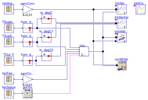
Validation model for the cooling coil control subsequence with recorded data trends
Information
This model validates the cooling coil signal subsequence implemented
in Building 33 on the main LBNL campus. Data used for the validation are measured
input and output trends with 5s time steps, starting at
2018-06-07 00:00:00 PDT. The trends were exported from the ALC EIKON webserver.
Extends from Modelica.Icons.Example (Icon for runnable examples).
Modelica definition
model ControlsVerification_CoolingCoilValve
extends Modelica.Icons.Example;
Modelica.Blocks.Sources.CombiTimeTable TOut_F(
tableOnFile=true,
extrapolation=Modelica.Blocks.Types.Extrapolation.Periodic,
offset={0},
timeScale(displayUnit="s"),
tableName="OA_Temp",
smoothness=Modelica.Blocks.Types.Smoothness.LinearSegments,
columns={3},
fileName=
Modelica.Utilities.Files.loadResource(
"modelica://Buildings/Resources/Data/Utilities/Plotters/Examples/ControlsVerification_CoolingCoilValve/OA_Temp.mos"))
;
Modelica.Blocks.Sources.CombiTimeTable TSupSetpoint_F(
tableOnFile=true,
extrapolation=Modelica.Blocks.Types.Extrapolation.Periodic,
offset={0},
timeScale(displayUnit="s"),
smoothness=Modelica.Blocks.Types.Smoothness.LinearSegments,
tableName="SA_Clg_Stpt",
columns={3},
fileName=
Modelica.Utilities.Files.loadResource(
"modelica://Buildings/Resources/Data/Utilities/Plotters/Examples/ControlsVerification_CoolingCoilValve/SA_Clg_Stpt.mos"))
;
Modelica.Blocks.Sources.CombiTimeTable coolingValveSignal(
tableOnFile=true,
extrapolation=Modelica.Blocks.Types.Extrapolation.Periodic,
offset={0},
timeScale(displayUnit="s"),
tableName="Clg_Coil_Valve",
columns={3},
smoothness=Modelica.Blocks.Types.Smoothness.LinearSegments,
fileName=
Modelica.Utilities.Files.loadResource(
"modelica://Buildings/Resources/Data/Utilities/Plotters/Examples/ControlsVerification_CoolingCoilValve/Clg_Coil_Valve.mos"))
;
Modelica.Blocks.Sources.CombiTimeTable fanFeedback(
tableOnFile=true,
extrapolation=Modelica.Blocks.Types.Extrapolation.Periodic,
offset={0},
timeScale(displayUnit="s"),
tableName="VFD_Fan_Feedback",
columns={3},
smoothness=Modelica.Blocks.Types.Smoothness.LinearSegments,
fileName=
Modelica.Utilities.Files.loadResource(
"modelica://Buildings/Resources/Data/Utilities/Plotters/Examples/ControlsVerification_CoolingCoilValve/VFD_Fan_Feedback.mos"))
;
Modelica.Blocks.Sources.CombiTimeTable fanStatus(
tableOnFile=true,
extrapolation=Modelica.Blocks.Types.Extrapolation.Periodic,
offset={0},
timeScale(displayUnit="s"),
tableName="VFD_Fan_Enable",
columns={3},
smoothness=Modelica.Blocks.Types.Smoothness.LinearSegments,
fileName=
Modelica.Utilities.Files.loadResource(
"modelica://Buildings/Resources/Data/Utilities/Plotters/Examples/ControlsVerification_CoolingCoilValve/VFD_Fan_Enable.mos"))
;
Modelica.Blocks.Sources.CombiTimeTable TSupply_F(
tableOnFile=true,
extrapolation=Modelica.Blocks.Types.Extrapolation.Periodic,
offset={0},
timeScale(displayUnit="s"),
smoothness=Modelica.Blocks.Types.Smoothness.LinearSegments,
tableName="Supply_Air_Temp",
columns={3},
fileName=
Modelica.Utilities.Files.loadResource(
"modelica://Buildings/Resources/Data/Utilities/Plotters/Examples/ControlsVerification_CoolingCoilValve/Supply_Air_Temp.mos"))
;
Buildings.Utilities.Plotters.Examples.BaseClasses.CoolingCoilValve cooValSta(
reverseActing=false,
TSupHighLim(displayUnit="degC"),
TSupHigLim(displayUnit="degC"),
TOutDelta(displayUnit="degC"),
TOutCooCut(displayUnit="degC") = 50*(5/9) - 32*(5/9) + 273.15)
;
Buildings.Controls.OBC.CDL.Reals.GreaterThreshold greThr(t=0.5)
;
Buildings.Controls.OBC.CDL.Reals.MultiplyByParameter percConv(k=0.01)
;
Buildings.Controls.OBC.CDL.Reals.MultiplyByParameter percConv1(k=0.01)
;
Buildings.Controls.OBC.UnitConversions.From_degF from_degF
;
Buildings.Controls.OBC.UnitConversions.From_degF from_degF1
;
Buildings.Controls.OBC.UnitConversions.From_degF from_degF2
;
Buildings.Controls.OBC.UnitConversions.To_degC to_degC
;
Buildings.Controls.OBC.UnitConversions.To_degC to_degC1
;
Buildings.Controls.OBC.UnitConversions.To_degC to_degC2
;
protected
Buildings.Utilities.IO.Files.CSVWriter csvWriter(
samplePeriod=5,
nin=2,
headerNames={"Trended","Modeled"})
;
inner Buildings.Utilities.Plotters.Configuration plotConfiguration(
timeUnit=Buildings.Utilities.Plotters.Types.TimeUnit.hours,
activation=Buildings.Utilities.Plotters.Types.GlobalActivation.always,
samplePeriod=300,
fileName="coolingCoilValve_validationPlots.html")
;
Buildings.Utilities.Plotters.Scatter correlation(
n=1,
legend={"Modeled cooling valve signal"},
xlabel="Trended cooling valve signal",
title="Modeled result/recorded trend correlation")
;
Buildings.Utilities.Plotters.TimeSeries timSerRes(
n=2,
legend={"Cooling valve control signal, modeled","Cooling valve control signal, trended"},
title="Cooling valve control signal: reference trend vs. modeled result")
;
Buildings.Utilities.Plotters.TimeSeries timSerInp(
n=3,
legend={"Supply air temperature, [degC]","Supply air temperature setpoint, [degC]",
"Outdoor air temperature, [degC]"},
title="Trended input signals")
;
equation
connect(cooValSta.yCooVal, timSerRes.y[1]);
connect(cooValSta.yCooVal, correlation.y[1]);
connect(percConv.y, timSerRes.y[2]);
connect(percConv.y, correlation.x);
connect(greThr.y, cooValSta.uFanSta);
connect(percConv1.y, cooValSta.uFanFee);
connect(coolingValveSignal.y[1], percConv.u);
connect(fanFeedback.y[1], percConv1.u);
connect(fanStatus.y[1], greThr.u);
connect(percConv.y,csvWriter. u[1]);
connect(cooValSta.yCooVal,csvWriter. u[2]);
connect(TSupply_F.y[1], from_degF.u);
connect(from_degF.y, to_degC.u);
connect(TSupSetpoint_F.y[1], from_degF1.u);
connect(from_degF1.y, to_degC1.u);
connect(TOut_F.y[1], from_degF2.u);
connect(from_degF2.y, to_degC2.u);
connect(from_degF2.y, cooValSta.TOut);
connect(from_degF1.y, cooValSta.TSupSet);
connect(from_degF.y, cooValSta.TSup);
connect(to_degC.y, timSerInp.y[1]);
connect(to_degC1.y, timSerInp.y[2]);
connect(to_degC2.y, timSerInp.y[3]);
end ControlsVerification_CoolingCoilValve;
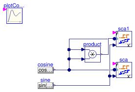
Simple scatter plots
Information
This example demonstrates the use of a scatter plotter
that plots (sin(t), cos(t)), which will be a circle
with radius 1,
and (sin(t), cos2(t)), which will be an arc
above the x-axis.
The plots will be in the file specified
in the plot configuration plotConfiguration.
Extends from Modelica.Icons.Example (Icon for runnable examples).
Modelica definition
model Scatter
extends Modelica.Icons.Example;
inner Buildings.Utilities.Plotters.Configuration plotConfiguration(
samplePeriod=0.1) ;
Buildings.Utilities.Plotters.Scatter sca(
samplePeriod=0.1,
n=1,
title="Sine vs cosine",
xlabel="sine",
legend={"cos"},
introduction="This plot shows a scatter plot of sine vs cosine.")
;
Modelica.Blocks.Sources.RealExpression sine(y=
sin(uniCon*time))
;
Modelica.Blocks.Sources.RealExpression cosine(y=
cos(uniCon*time))
;
Buildings.Utilities.Plotters.Scatter sca1(
samplePeriod=0.1,
n=2,
title="Sine vs cosine and sine vs cosine^2",
legend={"sin vs cos","sin vs cos^2"},
xlabel="sine",
introduction=
"This plot shows a scatter plot of sine vs cosine and of sine vs cosine^2.")
;
Modelica.Blocks.Math.Product product
;
protected
constant Real uniCon(
final unit="1/s") = 1
;
equation
connect(sca.x, sine.y);
connect(cosine.y, sca.y[1]);
connect(sca1.x, sine.y);
connect(cosine.y, sca1.y[1]);
connect(cosine.y, product.u1);
connect(cosine.y, product.u2);
connect(product.y, sca1.y[2]);
end Scatter;
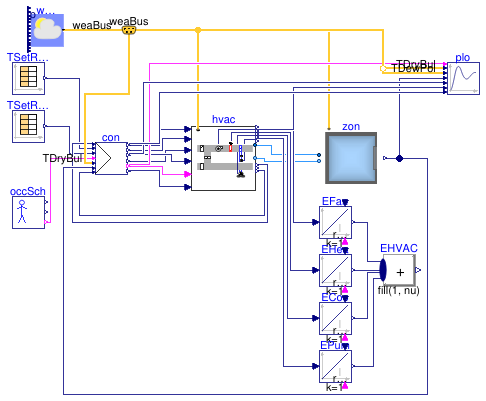
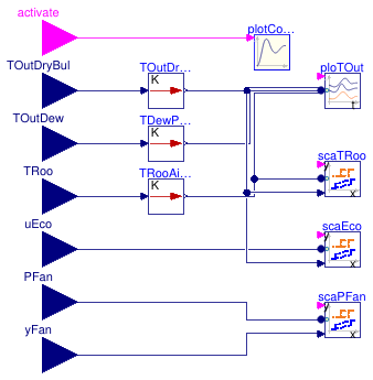
Various plots for a single zone VAV system
Information
This example demonstrates the use of a time plot and a scatter plot
for a single zone VAV system.
The plots are configured to plot every 15 minutes.
The plots will be in the file specified
in the plot configuration plotConfiguration.
Extends from Buildings.Air.Systems.SingleZone.VAV.Examples.ChillerDXHeatingEconomizer (Variable air volume flow system with single themal zone and conventional control).
Parameters
| Type | Name | Default | Description |
|---|
| Temperature | TSupChi_nominal | 279.15 | Design value for chiller leaving water temperature [K] |
Connectors
| Type | Name | Description |
|---|
| Bus | weaBus | Weather bus |
Modelica definition
model SingleZoneVAV
extends Buildings.Air.Systems.SingleZone.VAV.Examples.ChillerDXHeatingEconomizer;
Plotters plo ;
model Plotters
extends Modelica.Blocks.Icons.Block;
Modelica.Blocks.Interfaces.BooleanInput activate
;
Modelica.Blocks.Interfaces.RealInput TOutDryBul ;
Modelica.Blocks.Interfaces.RealInput TOutDew ;
Modelica.Blocks.Interfaces.RealInput TRoo ;
Modelica.Blocks.Interfaces.RealInput uEco ;
Modelica.Blocks.Interfaces.RealInput PFan ;
Modelica.Blocks.Interfaces.RealInput yFan ;
inner Buildings.Utilities.Plotters.Configuration plotConfiguration(
samplePeriod(displayUnit="min") = 900,
timeUnit=Buildings.Utilities.Plotters.Types.TimeUnit.days,
activation=Buildings.Utilities.Plotters.Types.GlobalActivation.use_input,
activationDelay(displayUnit="min") = 600)
;
Buildings.Utilities.Plotters.TimeSeries ploTOut(
title="Outdoor drybulb and dew point temperatures",
legend={"TOutDryBul","TOutDewPoi","TRoo"},
activation=Buildings.Utilities.Plotters.Types.LocalActivation.always,
introduction="Outside conditions.",
n=3) ;
Buildings.Utilities.Plotters.Scatter scaEco(
title="Economizer control signal",
legend={"uEco"},
xlabel="TOut [degC]",
n=1,
introduction="Economizer control signal while the system is operating for at least 10 minutes.")
;
Buildings.Utilities.Plotters.Scatter scaPFan(
title="Fan power",
xlabel="yFan [1]",
legend={"PFan in [W]"},
n=1,
activation=Buildings.Utilities.Plotters.Types.LocalActivation.always)
;
Buildings.Utilities.Plotters.Scatter scaTRoo(
xlabel="TOut [degC]",
title="Room air temperature",
legend={"TRoo [degC]"},
introduction="Room air temperatures while the system is operating for at least 10 minutes.",
n=1)
;
Modelica.Blocks.Math.UnitConversions.To_degC TRooAir_degC
;
Modelica.Blocks.Math.UnitConversions.To_degC TDewPoi_degC
;
Modelica.Blocks.Math.UnitConversions.To_degC TOutDryBul_degC
;
equation
connect(plotConfiguration.activate, activate);
connect(scaEco.y[1], uEco);
connect(scaPFan.x, yFan);
connect(PFan, scaPFan.y[1]);
connect(scaEco.x, TOutDryBul_degC.y);
connect(TOutDryBul_degC.u, TOutDryBul);
connect(TOutDew, TDewPoi_degC.u);
connect(TRoo, TRooAir_degC.u);
connect(TOutDryBul_degC.y, ploTOut.y[1]);
connect(TDewPoi_degC.y, ploTOut.y[2]);
connect(TRooAir_degC.y, ploTOut.y[3]);
connect(TRooAir_degC.y, scaTRoo.y[1]);
connect(scaTRoo.x, TOutDryBul_degC.y);
end Plotters;
equation
connect(plo.activate, con.chiOn);
connect(weaBus.TDryBul, plo.TOutDryBul);
connect(weaBus.TDewPoi, plo.TOutDew);
connect(plo.TRoo, zon.TRooAir);
connect(con.yOutAirFra, plo.uEco);
connect(hvac.PFan, plo.PFan);
connect(con.yFan, plo.yFan);
end SingleZoneVAV;
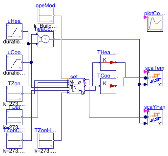
Scatter plots for control signal of a single zone VAV controller from ASHRAE Guideline 36
Information
This example demonstrates how to create a scatter plot that shows
for a single zone VAV control logic
the heating and cooling set point temperatures, and the fan speed,
all as a function of the heating and cooling control signal.
The sequence that will be used to plot the sequence diagram is
Buildings.Controls.OBC.ASHRAE.G36.AHUs.SingleZone.VAV.SetPoints.Supply
and shown below.
The plot will be generated in the file plots.html.

Extends from Modelica.Icons.Example (Icon for runnable examples).
Modelica definition
model SingleZoneVAVSupply_u
extends Modelica.Icons.Example;
inner Configuration plotConfiguration(samplePeriod=1) ;
Buildings.Controls.OBC.CDL.Reals.Subtract heaCooConSig
;
Buildings.Utilities.Plotters.Scatter scaTem(
title="Temperature setpoints",
n=2,
xlabel="Heating (negative) and cooling (positive) control loop signal",
legend={"THea [degC]","TCoo [degC]"},
introduction="Set point temperatures as a function of the heating loop signal (from -1 to 0) and
the cooling loop signal (from 0 to +1).")
;
Buildings.Controls.OBC.UnitConversions.To_degC THea_degC
;
Buildings.Controls.OBC.UnitConversions.To_degC TCoo_degC
;
Buildings.Utilities.Plotters.Scatter scaYFan(
n=1,
title="Fan control signal",
legend={"yFan"},
xlabel="Heating (negative) and cooling (positive) control loop signal",
introduction="Fan speed as a function of the heating loop signal (from -1 to 0) and
the cooling loop signal (from 0 to +1).")
;
Buildings.Controls.OBC.ASHRAE.G36.AHUs.SingleZone.VAV.SetPoints.Supply setPoiVAV(
maxHeaSpe=0.7,
maxCooSpe=1,
minSpe=0.3,
TSupDew_max=290.15,
TSup_max=303.15,
TSup_min=289.15)
;
Buildings.Controls.OBC.CDL.Reals.Sources.Constant TZon(
k = 273.15 + 28)
;
Buildings.Controls.OBC.CDL.Reals.Sources.Constant TOut(k=273.15 + 22)
;
Buildings.Controls.OBC.CDL.Reals.Sources.Ramp uHea(
duration=900,
height=-1,
offset=1) ;
Buildings.Controls.OBC.CDL.Reals.Sources.Ramp uCoo(duration=900,
startTime=2700)
;
Controls.OBC.CDL.Integers.Sources.Constant opeMod(
final k=Buildings.Controls.OBC.ASHRAE.G36.Types.OperationModes.occupied)
;
Controls.OBC.CDL.Reals.Sources.Constant TZonCooSet(
final k=
273.15 + 24)
;
Controls.OBC.CDL.Reals.Sources.Constant TZonHeaSet(
final k=
273.15 + 20)
;
equation
connect(TOut.y, setPoiVAV.TOut);
connect(uHea.y, setPoiVAV.uHea);
connect(uCoo.y, setPoiVAV.uCoo);
connect(scaTem.x, heaCooConSig.y);
connect(THea_degC.y, scaTem.y[1]);
connect(TCoo_degC.y, scaTem.y[2]);
connect(setPoiVAV.y, scaYFan.y[1]);
connect(heaCooConSig.y, scaYFan.x);
connect(setPoiVAV.TZon, TZon.y);
connect(uHea.y, heaCooConSig.u2);
connect(uCoo.y, heaCooConSig.u1);
connect(setPoiVAV.TSupCooSet, TCoo_degC.u);
connect(setPoiVAV.TSupHeaEcoSet, THea_degC.u);
connect(opeMod.y, setPoiVAV.uOpeMod);
connect(TZonCooSet.y, setPoiVAV.TCooSet);
connect(TZonHeaSet.y, setPoiVAV.THeaSet);
end SingleZoneVAVSupply_u;
Simple time series plots
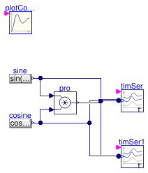
Information
This example demonstrates the use of a plotter
that plots (t, sin(t), cos(t), sin(t)*cos(t)) in
one plot, and
(t, sin(t), cos(t))
in another plot.
Both plots will be in the file specified
in the plot configuration plotConfiguration.
Extends from Modelica.Icons.Example (Icon for runnable examples).
Modelica definition
model TimeSeries
extends Modelica.Icons.Example;
inner Buildings.Utilities.Plotters.Configuration plotConfiguration(
samplePeriod=0.1,
timeUnit=Buildings.Utilities.Plotters.Types.TimeUnit.seconds)
;
Buildings.Utilities.Plotters.TimeSeries timSer(
samplePeriod=0.1,
n=3,
title="Sine, cosine and sine*cosine",
legend={"sin","cos","sin*cos"})
;
Modelica.Blocks.Sources.RealExpression sine(y=
sin(uniCon*time)) ;
Modelica.Blocks.Sources.RealExpression cosine(y=
cos(uniCon*time))
;
Buildings.Utilities.Plotters.TimeSeries timSer1(
samplePeriod=0.1,
n=2,
title="Sine, cosine",
legend={"sin","cos"})
;
Modelica.Blocks.Math.Product pro ;
protected
constant Real uniCon(
final unit="1/s") = 1
;
equation
connect(sine.y, timSer.y[1]);
connect(cosine.y, timSer.y[2]);
connect(sine.y, timSer1.y[1]);
connect(cosine.y, timSer1.y[2]);
connect(sine.y, pro.u1);
connect(cosine.y, pro.u2);
connect(pro.y, timSer.y[3]);
end TimeSeries;
Information
Block that contains unit conversion, plotter configuration
and various plotters.
Extends from Modelica.Blocks.Icons.Block (Basic graphical layout of input/output block).
Connectors
| Type | Name | Description |
|---|
| input BooleanInput | activate | Set to true to enable plotting of time series after activationDelay elapsed |
| input RealInput | TOutDryBul | Outdoor drybulb temperature |
| input RealInput | TOutDew | Outdoor dewpoint temperature |
| input RealInput | TRoo | Room temperature |
| input RealInput | uEco | Economizer control signal |
| input RealInput | PFan | Fan power consumption |
| input RealInput | yFan | Fan control signal |
Modelica definition
model Plotters
extends Modelica.Blocks.Icons.Block;
Modelica.Blocks.Interfaces.BooleanInput activate
;
Modelica.Blocks.Interfaces.RealInput TOutDryBul ;
Modelica.Blocks.Interfaces.RealInput TOutDew ;
Modelica.Blocks.Interfaces.RealInput TRoo ;
Modelica.Blocks.Interfaces.RealInput uEco ;
Modelica.Blocks.Interfaces.RealInput PFan ;
Modelica.Blocks.Interfaces.RealInput yFan ;
inner Buildings.Utilities.Plotters.Configuration plotConfiguration(
samplePeriod(displayUnit="min") = 900,
timeUnit=Buildings.Utilities.Plotters.Types.TimeUnit.days,
activation=Buildings.Utilities.Plotters.Types.GlobalActivation.use_input,
activationDelay(displayUnit="min") = 600)
;
Buildings.Utilities.Plotters.TimeSeries ploTOut(
title="Outdoor drybulb and dew point temperatures",
legend={"TOutDryBul","TOutDewPoi","TRoo"},
activation=Buildings.Utilities.Plotters.Types.LocalActivation.always,
introduction="Outside conditions.",
n=3) ;
Buildings.Utilities.Plotters.Scatter scaEco(
title="Economizer control signal",
legend={"uEco"},
xlabel="TOut [degC]",
n=1,
introduction="Economizer control signal while the system is operating for at least 10 minutes.")
;
Buildings.Utilities.Plotters.Scatter scaPFan(
title="Fan power",
xlabel="yFan [1]",
legend={"PFan in [W]"},
n=1,
activation=Buildings.Utilities.Plotters.Types.LocalActivation.always)
;
Buildings.Utilities.Plotters.Scatter scaTRoo(
xlabel="TOut [degC]",
title="Room air temperature",
legend={"TRoo [degC]"},
introduction="Room air temperatures while the system is operating for at least 10 minutes.",
n=1)
;
Modelica.Blocks.Math.UnitConversions.To_degC TRooAir_degC
;
Modelica.Blocks.Math.UnitConversions.To_degC TDewPoi_degC
;
Modelica.Blocks.Math.UnitConversions.To_degC TOutDryBul_degC
;
equation
connect(plotConfiguration.activate, activate);
connect(scaEco.y[1], uEco);
connect(scaPFan.x, yFan);
connect(PFan, scaPFan.y[1]);
connect(scaEco.x, TOutDryBul_degC.y);
connect(TOutDryBul_degC.u, TOutDryBul);
connect(TOutDew, TDewPoi_degC.u);
connect(TRoo, TRooAir_degC.u);
connect(TOutDryBul_degC.y, ploTOut.y[1]);
connect(TDewPoi_degC.y, ploTOut.y[2]);
connect(TRooAir_degC.y, ploTOut.y[3]);
connect(TRooAir_degC.y, scaTRoo.y[1]);
connect(scaTRoo.x, TOutDryBul_degC.y);
end Plotters;
 Buildings.Utilities.Plotters.Examples.ControlsVerification_CoolingCoilValve
 Buildings.Utilities.Plotters.Examples.SingleZoneVAV.Plotters