Buildings.Fluid.Movers.BaseClasses.Euler

Functions and data record templates for Euler number

Information

This package implements a power computation using the Euler number and its correlation.

The correlation function using the Euler number is implemented in Buildings.Fluid.Movers.BaseClasses.Euler.correlation.
When curves of power and pressure against flow rate is available, the function Buildings.Fluid.Movers.BaseClasses.Euler.getPeak can identify the peak operating condition from them. This is useful comparing power computation results against other methods.
The peak operating condition (where the efficiency η is at its maximum) which is used by the correlation is stored in an instance of the record Buildings.Fluid.Movers.BaseClasses.Euler.peak.
Buildings.Fluid.Movers.BaseClasses.FlowMachineInterface uses the peak values and the correlation to generate a power curve against volumetric flow rate. This estimated power curve is used in place of the measured power that would otherwise be provided.

See the User's Guide for more information.

Package Content

Name	Description
correlation	Correlation of static efficiency ratio vs log of Euler number ratio
efficiency	Computes efficiency with the Euler number correlation
getPeak	Find peak condition from power characteristics
power	Computes power as well as its derivative with respect to flow rate using Euler number
peak	Record for the operation condition at peak efficiency
powerWithDerivative	Record for electrical power and its derivative with respect to flow rate

Buildings.Fluid.Movers.BaseClasses.Euler.correlation

Correlation of static efficiency ratio vs log of Euler number ratio

Information

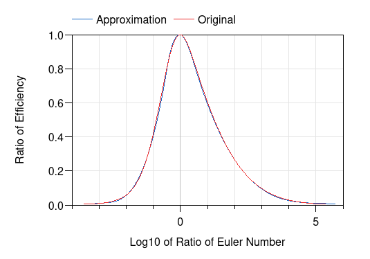
This function approximates the following correlation:

where y=η ⁄ η_p (note that η refers to the hydraulic efficiency instead of total efficiency), x=log₁₀(Eu ⁄ Eu_p), with the subscript p denoting the condition where the mover is operating at peak efficiency, and

Z₁=(x-a) ⁄ b

Z₂=(e^c⋅x⋅d⋅x-a) ⁄ b

Z₃=-a ⁄ b

a=-2.732094

b=2.273014

c=0.196344

d=5.267518

The approximation uses two simple polynomials stitched together by a third one of the same order. Care has been taken to ensure that, on the curve constructed by if statements, the differences of dy ⁄ dx evaluated by different groups of coefficients at the connecting points (i.e. at x = - 0.5 and x = + 0.5) are less than 1E-14. This way, the derivative is still continuous to the solver even if the solver requires a precision of 1E-10 when there are nested loops.

The correlation and the approximation have the shape as shown below (plotted by Buildings.Fluid.Movers.BaseClasses.Validation.EulerCurve).

The modified dimensionless Euler number is defined as

Eu=(Δp⋅D⁴) ⁄ (ρ⋅V̇²)

where Δp is the fan pressure rise in Pa, D is the fan wheel outer diameter in m, ρ is the inlet air density in kg/m³, and V̇ is the volumetric flow rate in m³/s. Note that the units in the definition do not matter to this correlation because it is the ratio of the Euler numbers that is used. Since D is constant for the same mover and ρ is approximately constant for common HVAC applications, the Euler number ratio can be simplified to

Eu ⁄ Eu_p=(Δp⋅V̇_p²) ⁄ (Δp_p⋅V̇²)

References

For more information regarding the correlation curve refer to EnergyPlus 9.6.0 Engineering Reference chapter 16.4 equations 16.209 through 16.218. Note that the formula is simplified here from the source document.

Resources

The svg file for the correlation equation was generated on https://viereck.ch/latex-to-svg using this script.

Extends from Modelica.Icons.Function (Icon for functions).

Inputs

Type	Name	Default	Description
Real	x		log10(Eu/Eu_peak)

Outputs

Type	Name	Description
Real	y	eta/eta_peak

Modelica definition

function correlation "Correlation of static efficiency ratio vs log of Euler number ratio" extends Modelica.Icons.Function; input Real x "log10(Eu/Eu_peak)"; output Real y "eta/eta_peak"; protected Real a "Polynomial coefficient"; Real b "Polynomial coefficient"; Real c "Polynomial coefficient"; Real d "Polynomial coefficient"; Real y1 "eta/eta_peak"; algorithm if x < -0.5 then a := 0.05687322707407; b := 0.493231336746; c := 1.433531254001; d := 1.407887300933; elseif x > 0.5 then a := -8.5494313567465000E-3; b := 1.2957001502368300E-1; c := -6.5997315029278200E-1; d := 1.13993003013131; else a := 0.37824577860088; b := -0.75988502317361; c := -0.060614519563716; d := 1.01426507307139; end if; y1 := (a*x^3 + b*x^2 + c*x + d) / 1.01545; // y1 is almost always bounded away from zero, // hence we make a test to see whether we indeed // need to call smoothMax or can avoid its overhead y := if y1 > 0.002 then y1 else Buildings.Utilities.Math.Functions.smoothMax( x1=y1, x2=0.001, deltaX=0.0005); end correlation;

Buildings.Fluid.Movers.BaseClasses.Euler.efficiency

Computes efficiency with the Euler number correlation

Information

This function uses the correlation of Euler number to compute the efficiency η.

Extends from Modelica.Icons.Function (Icon for functions).

Inputs

Type	Name	Description
peak	peak	Operation point with maximum efficiency
PressureDifference	dp	Pressure rise [Pa]
VolumeFlowRate	V_flow	Volumetric flow rate [m3/s]
Real	V_flow_dp_small	Small number for regularisation [m3.Pa/s]

Outputs

Type	Name	Description
Efficiency	eta	Efficiency [1]

Modelica definition

function efficiency "Computes efficiency with the Euler number correlation" extends Modelica.Icons.Function; input Buildings.Fluid.Movers.BaseClasses.Euler.peak peak "Operation point with maximum efficiency"; input Modelica.Units.SI.PressureDifference dp "Pressure rise"; input Modelica.Units.SI.VolumeFlowRate V_flow "Volumetric flow rate"; input Real V_flow_dp_small( final unit="m3.Pa/s", min = Modelica.Constants.eps) "Small number for regularisation"; output Modelica.Units.SI.Efficiency eta "Efficiency"; protected Real log_r_Eu "Log10 of Eu/Eu_peak"; algorithm log_r_Eu:= log10( Buildings.Utilities.Math.Functions.smoothMax( x1=dp * peak.V_flow^2, x2=V_flow_dp_small, deltaX=V_flow_dp_small/2) /Buildings.Utilities.Math.Functions.smoothMax( x1=peak.dp * V_flow^2, x2=V_flow_dp_small, deltaX=V_flow_dp_small/2)); eta:= peak.eta* Buildings.Fluid.Movers.BaseClasses.Euler.correlation(x=log_r_Eu); end efficiency;

Buildings.Fluid.Movers.BaseClasses.Euler.getPeak

Find peak condition from power characteristics

Information

This function finds or estimates the peak point (V̇,Δp,η)|η=η_max from the input power curve P(V̇) and pressure curve Δp(V̇) which may or may not contain non-zero values. The results are output as an instance of Buildings.Fluid.Movers.BaseClasses.Euler.peak. There are the following branches of computation based on information provided to the function:

If Δp(V̇) is unavailable, the function simply outputs (0,0,0.7).
If Δp(V̇) is provided but P(V̇) is unavailable, the function provides an estimation of the peak point at half of max flow rate (V̇_max ⁄ 2, Δp(V̇=V̇_max ⁄ 2), 0.7).
If both Δp(V̇) and P(V̇) are available, the function first computes η(V̇)=V̇ Δp ⁄ P.
- If η(V̇) has less than four data points or is monotonic, use one of the two which ever produces a higher η:
  - The interpolated point at half of max flow rate (V̇_max ⁄ 2, Δp(V̇=V̇_max ⁄ 2), η(V̇=V̇_max ⁄ 2))
  - The available point with the highest computed efficiency.
- Otherwise, the function runs a quartic regression on η(V̇) then solves its derivative to find an extremum. It assumes that there is only one extremum on the open interval (0,V̇_max).

Extends from Modelica.Icons.Function (Icon for functions).

Inputs

Type	Name	Default	Description
flowParameters	pressure		Pressure vs. flow rate
powerParameters	power		Power vs. flow rate

Outputs

Type	Name	Description
peak	peak	Operation point at maximum efficiency

Modelica definition

function getPeak "Find peak condition from power characteristics" extends Modelica.Icons.Function; input Buildings.Fluid.Movers.BaseClasses.Characteristics.flowParameters pressure "Pressure vs. flow rate"; input BaseClasses.Characteristics.powerParameters power "Power vs. flow rate"; output Buildings.Fluid.Movers.BaseClasses.Euler.peak peak "Operation point at maximum efficiency"; protected parameter Integer nPre = size(pressure.V_flow, 1) "Size of the pressure array"; parameter Integer nPow = size(power.V_flow, 1) "Size of the power array"; parameter Integer n = max(nPre, nPow) "Bigger of the two arrays"; parameter Modelica.Units.SI.VolumeFlowRate V_flow_hal= if max(pressure.V_flow) < 1E-6 then 0 else (pressure.V_flow[nPre] -(pressure.V_flow[nPre] - pressure.V_flow[nPre - 1]) /(pressure.dp[nPre] - pressure.dp[nPre - 1]) * pressure.dp[nPre])/2 "Half of max flow, max flow is where dp=0"; parameter Modelica.Units.SI.PressureDifference dpHalFlo= if max(pressure.V_flow) < 1E-6 then 0 else Buildings.Utilities.Math.Functions.smoothInterpolation( x=V_flow_hal, xSup=pressure.V_flow, ySup=pressure.dp, ensureMonotonicity=true) "Pressure rise at half flow"; Modelica.Units.SI.VolumeFlowRate V_flow[n] "Flow rate"; Modelica.Units.SI.PressureDifference dp[n] "Pressure rise"; Modelica.Units.SI.Power P[n] "Power"; Real eta[n] "Efficiency series"; Boolean etaLes "Efficiency series has less than four points"; Boolean etaMon "Efficiency series is monotonic"; // A b = y Real A[n,5] "Design matrix"; Real b[5] "Parameter vector"; Real r[3,2] "Roots"; algorithm if max(pressure.V_flow) < 1E-6 and max(pressure.dp) < 1E-6 then // If there is no pressure curve, no estimation can be made peak.V_flow:=0; peak.dp:=0; peak.eta:=0.7; elseif max(power.P) < 1E-6 then // If a pressure curve is available, but no power curve, // peak.V_flow = V_flow_max / 2, // peak.dp = dp(V_flow = V_flow_max / 2) peak.V_flow:=V_flow_hal; peak.dp:=dpHalFlo; peak.eta:=0.7; else // Both a pressure curve and a power curve are available. // Create arrays of the equal size if nPre == nPow then V_flow:= pressure.V_flow; dp:= pressure.dp; P:= power.P; else if nPre > nPow then V_flow:= pressure.V_flow; dp:= pressure.dp; for i in 1:n loop P[i]:= Buildings.Utilities.Math.Functions.smoothInterpolation( x=V_flow[i], xSup=power.V_flow, ySup=power.P, ensureMonotonicity=false); end for; else V_flow:= power.V_flow; P:= power.P; for i in 1:n loop dp[i]:= Buildings.Utilities.Math.Functions.smoothInterpolation( x=V_flow[i], xSup=pressure.V_flow, ySup=pressure.dp, ensureMonotonicity=true); end for; end if; end if; // Compute efficiency array eta:=V_flow.*dp./P; etaLes:=n<4; etaMon:=Buildings.Utilities.Math.Functions.isMonotonic( x=eta, strict=false); if etaLes or etaMon then // If less than four data points are provided or the efficiency curve is // monotonic, use the one of two which has the higher efficiency: // 1. the interpolated point at half of max flow; // 2. the available point with the highest efficiency. peak.eta:=Buildings.Utilities.Math.Functions.smoothInterpolation( x=V_flow_hal, xSup=V_flow, ySup=eta, ensureMonotonicity= Buildings.Utilities.Math.Functions.isMonotonic(eta, strict=false)); if peak.eta>max(eta) then peak.V_flow:=V_flow_hal; peak.dp:=dpHalFlo; else peak.eta:=max(eta); for i in 1:n loop if abs(eta[i]-peak.eta)<1E-6 then peak.V_flow:=V_flow[i]; peak.dp:=dp[i]; end if; end for; end if; else // Constructs the matrix equation A b = y for quartic regression, where // A is a 5-by-n design matrix, // b is a parameter vector with length 5, // and y = eta is the response vector with length n. A[:,1]:=ones(n); // Avoids 0^0 for i in 2:5 loop A[:,i]:=V_flow[:].^(i-1); end for; b:=Modelica.Math.Matrices.leastSquares(A,eta); // Solve the derivative for the max eta and corresponding V_flow. // This assumes that there will only be one real solution // and it falls within the range of V_flow[:]. r:=Modelica.Math.Polynomials.roots({b[5]*4,b[4]*3,b[3]*2,b[2]}); for i in 1:3 loop if abs(r[i,2])<=1E-6 and r[i,1]>V_flow[1] and r[i,1]<V_flow[n] then peak.V_flow:=r[i,1]; end if; end for; peak.eta:=Buildings.Utilities.Math.Functions.smoothInterpolation( x=peak.V_flow, xSup=V_flow, ySup=eta, ensureMonotonicity=false); peak.dp:=Buildings.Utilities.Math.Functions.smoothInterpolation( x=peak.V_flow, xSup=V_flow, ySup=dp, ensureMonotonicity=false); end if; end if; end getPeak;

Buildings.Fluid.Movers.BaseClasses.Euler.power

Computes power as well as its derivative with respect to flow rate using Euler number

Information

This function outputs power values as well as its derivative versus volumetric flow rate in the following steps:

It first interpolates the input pressure curve to find a new pressure curve of 11 points on 10% increments of max flow rate. It assumes that the last point on the input pressure curve corresponds to Δp = 0, which is ensured when this function is called by Buildings.Fluid.Movers.BaseClasses.FlowMachineInterface.
It then computes power using efficiency evaluated with the Euler number from 10% to 90% of max flow rate on 10% increments.
With the incomplete power curve it computes the spline derivatives with respect to flow rate at the same points.
Once the derivatives are available, the power values at the two boundary points are found through linear extrapolation.

These steps are designed to ensure that power and efficiency computation with the Euler number is handled correctly near zero flow or zero pressure, where

Ẇ_flo = 0,
η = 0,
P > 0

in the equation

η = Ẇ_flo ⁄ P.

Extends from Modelica.Icons.Function (Icon for functions).

Inputs

Type	Name	Default	Description
peak	peak		Peak operation point
flowParametersInternal	pressure		Pressure curve with both max flow rate and max pressure

Outputs

Type	Name	Description
powerWithDerivative	power	Power and its derivative vs. flow rate

Modelica definition

function power "Computes power as well as its derivative with respect to flow rate using Euler number" extends Modelica.Icons.Function; input Buildings.Fluid.Movers.BaseClasses.Euler.peak peak "Peak operation point"; input Buildings.Fluid.Movers.BaseClasses.Characteristics.flowParametersInternal pressure "Pressure curve with both max flow rate and max pressure"; output Buildings.Fluid.Movers.BaseClasses.Euler.powerWithDerivative power( V_flow=zeros(11),P=zeros(11),d=zeros(11)) "Power and its derivative vs. flow rate"; protected Modelica.Units.SI.VolumeFlowRate V_flow[11] "Volumetric flow rate"; Modelica.Units.SI.PressureDifference dp[11] "Pressure rise"; Real V_flow_dp_small( final unit="m3.Pa/s", min = Modelica.Constants.eps) "Small value for regularisation"; algorithm // Construct pressure curve of 10% max flow rate increments // from the given pressure curve V_flow:={pressure.V_flow[end]*i*0.1 for i in 0:10}; for i in 1:11 loop dp[i]:=Buildings.Utilities.Math.Functions.smoothInterpolation( x=V_flow[i], xSup=pressure.V_flow, ySup=pressure.dp, ensureMonotonicity=false); end for; // Compute the power and derivative on non-boundary points // using efficiency estimated by Euler number method power.V_flow:=V_flow; V_flow_dp_small :=1E-4*max(pressure.V_flow)*max(pressure.dp); for i in 2:10 loop power.P[i]:=V_flow[i] * dp[i] / Buildings.Fluid.Movers.BaseClasses.Euler.efficiency( peak=peak, dp=dp[i], V_flow=V_flow[i], V_flow_dp_small=V_flow_dp_small/2); end for; power.d[2:10]:=Buildings.Utilities.Math.Functions.splineDerivatives( x=V_flow[2:10], y=power.P[2:10], ensureMonotonicity=false); // Use linear extrapolation to find the boundary points power.d[1]:=power.d[2]; power.d[11]:=power.d[10]; power.P[1]:=power.P[2]-power.d[2]*V_flow[2]; power.P[11]:=power.P[10]+power.d[10]*(V_flow[11]-V_flow[10]); end power;

Buildings.Fluid.Movers.BaseClasses.Euler.peak

Record for the operation condition at peak efficiency

Information

Record for performance data that describe the operation at peak efficiency.

Extends from Modelica.Icons.Record (Icon for records).

Parameters

Type	Name	Default	Description
VolumeFlowRate	V_flow		Volume flow rate at peak efficiency [m3/s]
PressureDifference	dp		Pressure rise at peak efficiency [Pa]
Efficiency	eta	0.7	Peak efficiency [1]

Modelica definition

record peak "Record for the operation condition at peak efficiency" extends Modelica.Icons.Record; parameter Modelica.Units.SI.VolumeFlowRate V_flow(min=0) "Volume flow rate at peak efficiency"; parameter Modelica.Units.SI.PressureDifference dp( min=0, displayUnit="Pa") "Pressure rise at peak efficiency"; parameter Modelica.Units.SI.Efficiency eta=0.7 "Peak efficiency"; end peak;

Buildings.Fluid.Movers.BaseClasses.Euler.powerWithDerivative

Record for electrical power and its derivative with respect to flow rate

Information

Data record for performance data that describe electrical power and its derivative versus volumetric flow rate. This record is specifically constructed for the Euler number method and is the output type of function Buildings.Fluid.Movers.BaseClasses.Euler.power.

Extends from Modelica.Icons.Record (Icon for records).

Parameters

Type	Name	Description
VolumeFlowRate	V_flow[11]	Volume flow rate at user-selected operating points [m3/s]
Power	P[11]	Fan or pump electrical power at these flow rates [W]
Real	d[11]	Derivative of power with respect to volume flow rate [J/m3]

Modelica definition

record powerWithDerivative "Record for electrical power and its derivative with respect to flow rate" extends Modelica.Icons.Record; parameter Modelica.Units.SI.VolumeFlowRate V_flow[11](each min=0) "Volume flow rate at user-selected operating points"; parameter Modelica.Units.SI.Power P[11](each min=0) "Fan or pump electrical power at these flow rates"; parameter Real d[11](each unit="J/m3") "Derivative of power with respect to volume flow rate"; end powerWithDerivative;