Package with aquifer thermal energy storage models
Information
Package with models for aquifer thermal energy storage.
Extends from Modelica.Icons.Package (Icon for standard packages).
Package Content
| Name |
Description |
 MultiWell MultiWell
|
Model of a single well for aquifer thermal energy storage |
 Data Data
|
Collection of data records for aquifer thermal energy storage |
 Examples Examples
|
Example models for Buildings.Fluid.Geothermal.Aquifer |
| Validation
|
Validation models for aquifer thermal energy storage |
Model of a single well for aquifer thermal energy storage
Information
This model simulates aquifer thermal energy storage, using one or multiple pairs of cold and hot wells.
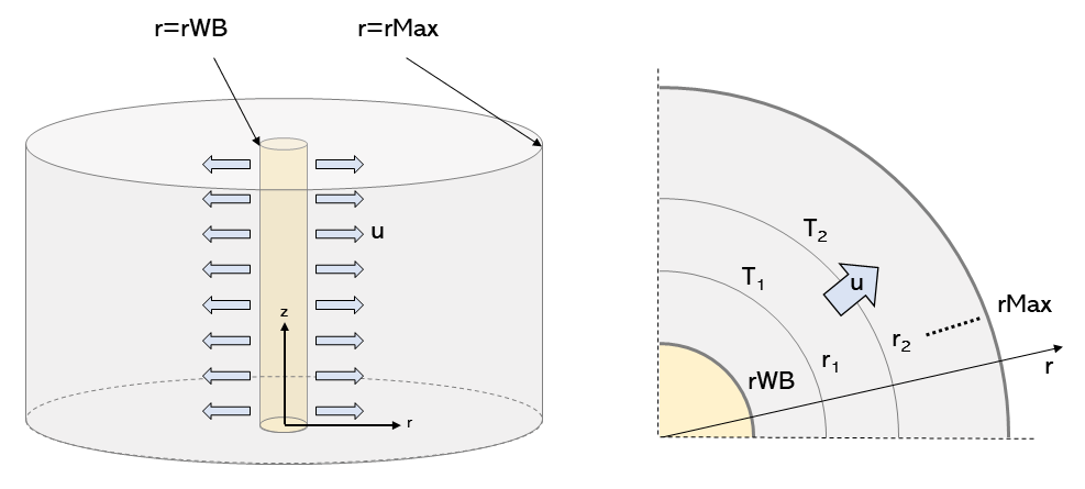
To calculate aquifer temperature at different locations over time, the model applies
physical principles of water flow and heat transfer phenomena. The model is based on
the partial differential equation (PDE) for 1D conductive-convective transient
radial heat transport in porous media
ρ c (∂ T(r,t) ⁄ ∂t) =
k (∂² T(r,t) ⁄ ∂r²) - ρw cw u(∂ T(r,t) ⁄ ∂t),
where
ρ
is the mass density,
c
is the specific heat capacity per unit mass,
T
is the temperature at location r and time t,
u is water velocity and
k is the heat conductivity. The subscript w indicates water.
The first term on the right hand side of the equation describes the effect of conduction, while
the second term describes the fluid flow.
The pressure losses in the aquifer are calculated using the Darcy's law
Δp = ṁ g ⁄ (2 π K h ln(rMax ⁄ rWB)),
where ṁ is the water mass flow rate, g is the gravitational acceleration,
K is the hydraulic conductivity, h is the thickness of the aquifer,
rMax is the domain radius and rWB is the well radius.
The pressure losses in the wells are calculated using
Modelica.Fluid.Pipes.BaseClasses.WallFriction.Detailed.pressureLoss_m_flow.
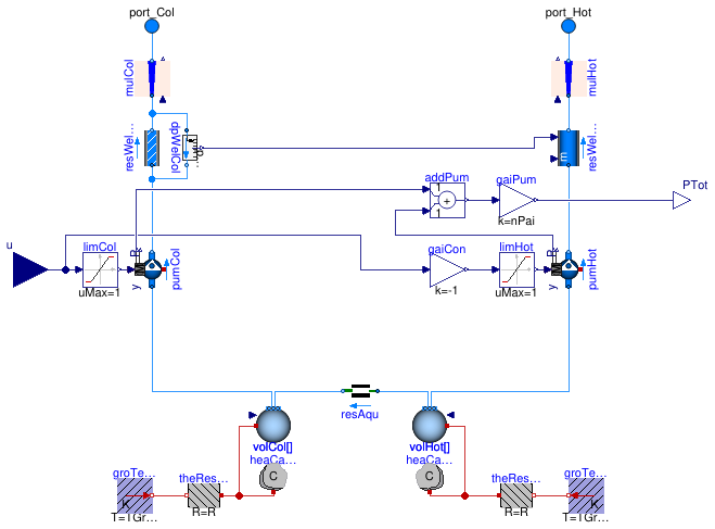
Spatial discretization
To discretize the conductive-convective equation, the domain is divided into a series
of thermal capacitances and thermal resistances along the radial direction. The
implementation uses an array of
Modelica.Thermal.HeatTransfer.Components.HeatCapacitor
and
Modelica.Thermal.HeatTransfer.Components.ThermalResistor.
Fluid flow was modelled by adding a series of fluid volumes, which are connected
to the thermal capacitances via heat ports. The fluid stream was developed using
the model Buildings.Fluid.MixingVolumes.MixingVolume.
The geometric representation of the model is illustrated in the figure below.
Typical use and important parameters
By default, the component consists of a single pair of wells: one cold well and one warm well.
The number of paired wells can be increased by modifing the parameters nPai.
The effect is a proportional increase of thermal capacity, and the mass flow rate at port_a
and port_b is equally distributed to the pairs of well, thus
all pairs have the same mass flow rates and temperatures, and the quantities
at the fluid ports is for all well combined, as is the electricity consumption PTot
for the well pumps.
To ensure conservation of energy, the wells are connected via fluid ports.
To avoid thermal interferences, make sure that the aquifer domain radius
rMax is large enough for your specific use case.
Circulation pumps are included in the model and they can be controlled by acting on the input connector.
The input must vary between [1, -1].
A positive value will circulate water
clockwise (from port_Hot to port_Col, thus
extraction from the cold well and injection into the warm well).
A negative value will circulate water anticlockwise.
The temperature values in the warm and cold aquifers can be accessed using
TAquHot and TAquCol.
These temperatures correspond to the temperatures of each thermal capacitance
in the discretized domain. The location of the thermal capacitance is expressed by rVol.
Implementation
The model computes the flow resistance of the cold well and the cold acquifer.
Because of symmetry, the warm side has the same flow resistances.
To reduce the number of equations in the model, the flow resistance of the warm
side is set to the same flow resistance as on the cold side, but with the
sign reversed.
Parameters
| Type | Name | Default | Description |
|---|
| replaceable package Medium | Modelica.Media.Interfaces.Pa... | Medium in the component |
| Height | h | | Aquifer thickness [m] |
| Length | d | | Distance between wells [m] |
| Height | length | | Length of one well, used to compute pressure drop [m] |
| Real | nPai | 1 | Number of paired wells |
| Template | aquDat | | Aquifer thermal properties |
| Subsurface |
| Integer | nVol | 10 | Number of control volumes used in discretization |
| Radius | rWB | 0.1 | Wellbore radius [m] |
| Radius | rMax | d/2 | Domain radius [m] |
| Real | griFac | 1.15 | Grid factor for spacing |
| Temperature | TCol_start | 283.15 | Initial temperature of cold well [K] |
| Temperature | THot_start | TCol_start | Initial temperature of warm well [K] |
| Properties of ground |
| Temperature | TGroCol | 285.15 | Undisturbed ground temperature (cold well) [K] |
| Temperature | TGroHot | TGroCol | Undisturbed ground temperature (warm well) [K] |
| Hydraulic circuit |
| MassFlowRate | m_flow_nominal | | Nominal mass flow rate [kg/s] |
| PressureDifference | dpAquifer_nominal | m_flow_nominal/nPai*Modelica... | Pressure drop at nominal mass flow rate in the aquifer [Pa] |
| PressureDifference | dpExt_nominal | | Pressure drop at nominal mass flow rate in the above-surface system (used to size the head of the well pump) [Pa] |
Connectors
| Type | Name | Description |
|---|
| replaceable package Medium | Medium in the component |
| input RealInput | u | Pump control input (-1: extract from hot well, +1: extract from cold well, 0: off) [1] |
| output RealOutput | PTot | Total power consumed by all circulation pumps in the wells [W] |
| FluidPort_a | port_Col | Fluid connector |
| FluidPort_a | port_Hot | Fluid connector |
Modelica definition
model MultiWell
replaceable package Medium =
Modelica.Media.Interfaces.PartialMedium ;
parameter Integer nVol(min=1)=10 ;
parameter Modelica.Units.SI.Height h ;
parameter Modelica.Units.SI.Length d ;
parameter Modelica.Units.SI.Height length
;
parameter Real nPai=1 ;
parameter Modelica.Units.SI.Radius rWB=0.1 ;
parameter Modelica.Units.SI.Radius rMax=d/2 ;
parameter Real griFac(min=1) = 1.15 ;
parameter Modelica.Units.SI.Temperature TCol_start=283.15
;
parameter Modelica.Units.SI.Temperature THot_start=TCol_start
;
parameter Modelica.Units.SI.Temperature TGroCol=285.15
;
parameter Modelica.Units.SI.Temperature TGroHot=TGroCol
;
parameter Buildings.Fluid.Geothermal.Aquifer.Data.Template aquDat
;
parameter Modelica.Units.SI.MassFlowRate m_flow_nominal ;
parameter Modelica.Units.SI.PressureDifference dpAquifer_nominal(displayUnit= "Pa")=
m_flow_nominal/nPai*Modelica.Constants.g_n/2/Modelica.Constants.pi/h/aquDat.K*
log(d/rWB)
;
final parameter Modelica.Units.SI.PressureDifference dpWell_nominal(
displayUnit="Pa") = 2*resWelCol.dp_nominal
;
parameter Modelica.Units.SI.PressureDifference dpExt_nominal(displayUnit="Pa")
;
final parameter Modelica.Units.SI.Radius rVol[nVol](
each final fixed=false)
;
Modelica.Blocks.Interfaces.RealInput u(
final min=-1,
final max=1,
final unit="1")
;
Modelica.Blocks.Interfaces.RealOutput PTot(
final unit="W")
;
Modelica.Fluid.Interfaces.FluidPort_a port_Col(
redeclare final package Medium =
Medium) ;
Modelica.Fluid.Interfaces.FluidPort_a port_Hot(
redeclare final package Medium =
Medium) ;
Modelica.Units.SI.Temperature TAquHot[nVol] = heaCapHot.T
;
Modelica.Units.SI.Temperature TAquCol[nVol] = heaCapCol.T
;
Movers.Preconfigured.SpeedControlled_y pumCol(
redeclare final package Medium =
Medium,
final m_flow_nominal=m_flow_nominal/nPai,
final dp_nominal=resAqu.dpMea_nominal + 2* resWelCol.dp_nominal + dpExt_nominal)
;
Movers.Preconfigured.SpeedControlled_y pumHot(
redeclare final package Medium =
Medium,
final m_flow_nominal=pumCol.m_flow_nominal,
final dp_nominal=pumCol.dp_nominal) ;
FixedResistances.PressureDrop resWelCol(
redeclare final package Medium =
Medium,
m_flow_nominal=m_flow_nominal/nPai,
final from_dp=false,
dp_nominal=
Modelica.Fluid.Pipes.BaseClasses.WallFriction.Detailed.pressureLoss_m_flow(
m_flow=m_flow_nominal/nPai,
rho_a=rhoWat,
rho_b=rhoWat,
mu_a=mu,
mu_b=mu,
length=length,
diameter=rWB,
roughness=2.5e-5)) ;
Movers.BaseClasses.IdealSource resWelHot(
redeclare final package Medium =
Medium,
final allowFlowReversal=true,
final control_m_flow=false,
final control_dp=true,
final m_flow_small=1E-4*
abs(m_flow_nominal))
;
BaseClasses.MassFlowRateMultiplier mulCol(
redeclare final package Medium =
Medium,
k=nPai)
;
BaseClasses.MassFlowRateMultiplier mulHot(
redeclare final package Medium =
Medium,
k=nPai)
;
Modelica.Blocks.Math.Add addPum(
final k1=1,
final k2=1)
;
Sensors.RelativePressure dpWelCol(
redeclare package Medium =
Medium)
;
Airflow.Multizone.Point_m_flow resAqu(
redeclare final package Medium =
Medium,
m=1,
final dpMea_nominal=dpAquifer_nominal,
final mMea_flow_nominal=m_flow_nominal/nPai)
;
protected
parameter Modelica.Units.SI.Radius r[nVol + 1](
each fixed=false)
;
parameter Modelica.Units.SI.HeatCapacity C[nVol](
each fixed=false)
;
parameter Modelica.Units.SI.Volume VWat[nVol](
each fixed=false)
;
parameter Modelica.Units.SI.ThermalResistance R[nVol](
each fixed=false)
;
parameter Real cAqu(fixed=false)
;
parameter Real kVol(fixed=false)
;
parameter Modelica.Units.SI.DynamicViscosity mu=
Medium.dynamicViscosity(
Medium.setState_pTX(
Medium.p_default,
Medium.T_default,
Medium.X_default)) ;
parameter Modelica.Units.SI.SpecificHeatCapacity cpWat=
Medium.specificHeatCapacityCp(
Medium.setState_pTX(
Medium.p_default,
Medium.T_default,
Medium.X_default)) ;
parameter Modelica.Units.SI.Density rhoWat=
Medium.density(
Medium.setState_pTX(
Medium.p_default,
Medium.T_default,
Medium.X_default)) ;
parameter Modelica.Units.SI.ThermalConductivity kWat=
Medium.thermalConductivity(
Medium.setState_pTX(
Medium.p_default,
Medium.T_default,
Medium.X_default)) ;
Buildings.Fluid.MixingVolumes.MixingVolume volCol[nVol](
redeclare final package Medium =
Medium,
each final T_start=TCol_start,
each final m_flow_nominal=m_flow_nominal,
final V=VWat,
each nPorts=2)
;
Modelica.Thermal.HeatTransfer.Components.HeatCapacitor heaCapCol[nVol](C=C,
each T(start=TCol_start, fixed=true))
;
Modelica.Thermal.HeatTransfer.Components.ThermalResistor theResCol[nVol](R=R)
;
MixingVolumes.MixingVolume volHot[nVol](
redeclare final package Medium =
Medium,
each T_start=THot_start,
each m_flow_nominal=m_flow_nominal,
V=VWat,
each nPorts=2)
;
Modelica.Thermal.HeatTransfer.Components.HeatCapacitor heaCapHot[nVol](C=C,
each T(start=THot_start, fixed=true))
;
Modelica.Thermal.HeatTransfer.Components.ThermalResistor theResHot[nVol](R=R)
;
Buildings.HeatTransfer.Sources.FixedTemperature groTemCol(
final T=TGroCol)
;
Buildings.HeatTransfer.Sources.FixedTemperature groTemHot(
final T=TGroHot)
;
Modelica.Blocks.Nonlinear.Limiter limCol(
final uMax=1,
final uMin=0) ;
Modelica.Blocks.Math.Gain gaiCon(
final k=-1) ;
Modelica.Blocks.Nonlinear.Limiter limHot(
final uMax=1,
final uMin=0) ;
Modelica.Blocks.Math.Gain gaiPum(
final k=nPai) ;
initial equation
assert(rWB < rMax, "In " +
getInstanceName() + ": Require rWB < rMax");
assert(0 < rWB, "In " +
getInstanceName() + ": Require 0 < rWB");
assert(rMax <= d/2, "In " +
getInstanceName() + ": Require rMax <= d/2");
cAqu=aquDat.dSoi*aquDat.cSoi*(1-aquDat.phi);
kVol=kWat*aquDat.phi+aquDat.kSoi*(1-aquDat.phi);
r[1] = rWB;
for i
in 2:nVol+1
loop
r[i]= r[i-1] + (rMax - rWB) * (1-griFac)/(1-griFac^(nVol)) * griFac^(i-2);
end for;
for i
in 1:nVol
loop
rVol[i] = (r[i]+r[i+1])/2;
end for;
for i
in 1:nVol
loop
C[i] = cAqu*h*3.14*(r[i+1]^2-r[i]^2);
end for;
for i
in 1:nVol
loop
VWat[i] = aquDat.phi*h*3.14*(r[i+1]^2-r[i]^2);
end for;
R[nVol]=
Modelica.Math.log(rMax/rVol[nVol])/(2*Modelica.Constants.pi*kVol*h);
for i
in 1:nVol-1
loop
R[i] =
Modelica.Math.log(rVol[i+1]/rVol[i])/(2*Modelica.Constants.pi*kVol*h);
end for;
equation
if nVol > 1
then
for i
in 1:(nVol - 1)
loop
connect(volCol[i].ports[2], volCol[i + 1].ports[1]);
end for;
end if;
connect(resAqu.port_b, volCol[nVol].ports[2]);
connect(resAqu.port_a, volHot[nVol].ports[2]);
connect(pumCol.port_a, volCol[1].ports[1]);
connect(pumHot.port_a, volHot[1].ports[1]);
if nVol > 1
then
for i
in 1:(nVol - 1)
loop
connect(volHot[i].ports[2], volHot[i + 1].ports[1]);
end for;
end if;
if nVol > 1
then
for i
in 1:(nVol - 1)
loop
connect(heaCapCol[i + 1].port, theResCol[i].port_b);
end for;
end if;
if nVol > 1
then
for i
in 1:(nVol - 1)
loop
connect(heaCapHot[i + 1].port, theResHot[i].port_b);
end for;
end if;
connect(groTemCol.port, theResCol[nVol].port_b);
connect(volCol.heatPort, heaCapCol.port);
connect(theResCol.port_a, volCol.heatPort);
connect(groTemHot.port, theResHot[nVol].port_b);
connect(volHot.heatPort, heaCapHot.port);
connect(theResHot.port_a, volHot.heatPort);
connect(pumCol.port_b, resWelCol.port_a);
connect(resWelHot.port_a, pumHot.port_b);
connect(limCol.y, pumCol.y);
connect(gaiCon.y, limHot.u);
connect(limHot.y, pumHot.y);
connect(gaiCon.u, u);
connect(limCol.u, u);
connect(resWelCol.port_b, mulCol.port_a);
connect(mulCol.port_b, port_Col);
connect(mulHot.port_b, port_Hot);
connect(resWelHot.port_b, mulHot.port_a);
connect(pumCol.P, addPum.u1);
connect(addPum.y, gaiPum.u);
connect(pumHot.P, addPum.u2);
connect(gaiPum.y, PTot);
connect(dpWelCol.port_a, resWelCol.port_b);
connect(dpWelCol.port_b, resWelCol.port_a);
connect(dpWelCol.p_rel, resWelHot.dp_in);
end MultiWell;
 Buildings.Fluid.Geothermal.Aquifer.MultiWell