Buildings.Utilities.Math.Functions.Examples

Information

This package contains examples for the use of models that can be found in Buildings.Utilities.Math.Functions.

Package Content

Name	Description
InverseXRegularized	Test problem for function that replaces 1/x around the origin by a twice continuously differentiable function
PolynomialDerivativeCheck
PowerLinearized	Test problem for function that linearizes y=x^n below some threshold
RegNonZeroPower
RegNonZeroPowerDerivative_2_Check
RegNonZeroPowerDerivativeCheck
SmoothExponentialDerivativeCheck
SpliceFunction
SpliceFunctionDerivativeCheck
CubicHermite	Test problem for cubic hermite splines

Buildings.Utilities.Math.Functions.Examples.InverseXRegularized

Information

Parameters

Type	Name	Default	Description
Real	delta	0.5	Small value for approximation

Modelica definition

model InverseXRegularized 
  "Test problem for function that replaces 1/x around the origin by a twice continuously differentiable function"
  extends Modelica.Icons.Example;
  Real x "Indepedent variable";
  parameter Real delta = 0.5 "Small value for approximation";
  Real y "Function value";
  Real xInv "Function value";
equation 
  x=2*time-1;
  xInv = if ( abs(x) > 0.1)   then 1 / x else 0;
  y = Buildings.Utilities.Math.Functions.inverseXRegularized(x=x, delta=delta);
end InverseXRegularized;

Buildings.Utilities.Math.Functions.Examples.PolynomialDerivativeCheck

Information

This example checks whether the function derivative is implemented correctly. If the derivative implementation is incorrect, the model will stop with an assert statement.

Modelica definition

model PolynomialDerivativeCheck
  extends Modelica.Icons.Example;
  Real x;
  Real y;
initial equation 
   y=x;
equation 
  x=Buildings.Utilities.Math.Functions.polynomial(x=time-2, a={2, 4, -4, 5});
  der(y)=der(x);
  // Trigger an error if the derivative implementation is incorrect.
  assert(abs(x-y) < 1E-2, "Model has an error.");

end PolynomialDerivativeCheck;

Buildings.Utilities.Math.Functions.Examples.PowerLinearized

Information

Modelica definition

model PowerLinearized 
  "Test problem for function that linearizes y=x^n below some threshold"
  extends Modelica.Icons.Example;
  Real T4(start=300^4) "Temperature raised to 4-th power";
  Real T "Temperature";
  Real TExact "Temperature";
equation 
  T = (1+500*time);
  T = Buildings.Utilities.Math.Functions.powerLinearized(x=T4, x0=243.15^4, n=0.25);
  TExact = abs(T4)^(1/4);

end PowerLinearized;

Buildings.Utilities.Math.Functions.Examples.RegNonZeroPower

Information

Modelica definition

model RegNonZeroPower
  extends Modelica.Icons.Example;
  Real y "Function value";
equation 
  y=Buildings.Utilities.Math.Functions.regNonZeroPower(
                                             time, 0.3, 0.5);
end RegNonZeroPower;

Buildings.Utilities.Math.Functions.Examples.RegNonZeroPowerDerivative_2_Check

Information

This example checks whether the function derivative is implemented correctly. If the derivative implementation is not correct, the model will stop with an assert statement.

Parameters

Type	Name	Default	Description
Real	n	0.33	Exponent
Real	delta	0.1	Abscissa value where transition occurs

Modelica definition

model RegNonZeroPowerDerivative_2_Check
  extends Modelica.Icons.Example;

 parameter Real n=0.33 "Exponent";
 parameter Real delta = 0.1 "Abscissa value where transition occurs";

  Real x;
  Real y;
initial equation 
   y=x;
equation 
  x=Buildings.Utilities.Math.Functions.BaseClasses.der_regNonZeroPower(
                                                             time,n, delta, time);
  der(y)=der(x);
  assert(abs(x-y) < 1E-2, "Model has an error");

end RegNonZeroPowerDerivative_2_Check;

Buildings.Utilities.Math.Functions.Examples.RegNonZeroPowerDerivativeCheck

Information

This example checks whether the function derivative is implemented correctly. If the derivative implementation is not correct, the model will stop with an assert statement.

Parameters

Type	Name	Default	Description
Real	n	0.33	Exponent
Real	delta	0.1	Abscissa value where transition occurs

Modelica definition

model RegNonZeroPowerDerivativeCheck
  extends Modelica.Icons.Example;
 parameter Real n=0.33 "Exponent";
 parameter Real delta = 0.1 "Abscissa value where transition occurs";

  Real x;
  Real y;
initial equation 
   y=x;
equation 
  x=Buildings.Utilities.Math.Functions.regNonZeroPower(
                                             time,n, delta);
  der(y)=der(x);
  assert(abs(x-y) < 1E-2, "Model has an error");

end RegNonZeroPowerDerivativeCheck;

Buildings.Utilities.Math.Functions.Examples.SmoothExponentialDerivativeCheck

Information

This example checks whether the function derivative is implemented correctly. If the derivative implementation is not correct, the model will stop with an assert statement.

Modelica definition

model SmoothExponentialDerivativeCheck
  extends Modelica.Icons.Example;

  Real x;
  Real y;
  Real ex "exact function value";
initial equation 
   y=x;
equation 
  x=Buildings.Utilities.Math.Functions.smoothExponential(
                                               x=time-2, delta=0.5);
  der(y)=der(x);
  assert(abs(x-y) < 1E-2, "Model has an error");
  ex=exp(-abs(time-2));
end SmoothExponentialDerivativeCheck;

Buildings.Utilities.Math.Functions.Examples.SpliceFunction

Information

Modelica definition

model SpliceFunction
  extends Modelica.Icons.Example;

  Real y "Function value";
equation 
  y=Buildings.Utilities.Math.Functions.spliceFunction(
                                            pos=10, neg=-10, x=time-0.4, deltax=0.2);
end SpliceFunction;

Buildings.Utilities.Math.Functions.Examples.SpliceFunctionDerivativeCheck

Information

This example checks whether the function derivative is implemented correctly. If the derivative implementation is not correct, the model will stop with an assert statement.

Modelica definition

model SpliceFunctionDerivativeCheck
  extends Modelica.Icons.Example;

  Real x;
  Real y;
initial equation 
   y=x;
equation 
  x=Buildings.Utilities.Math.Functions.spliceFunction(
                                            10, -10, time+0.1, 0.2);
  der(y)=der(x);
  assert(abs(x-y) < 1E-2, "Model has an error");

end SpliceFunctionDerivativeCheck;

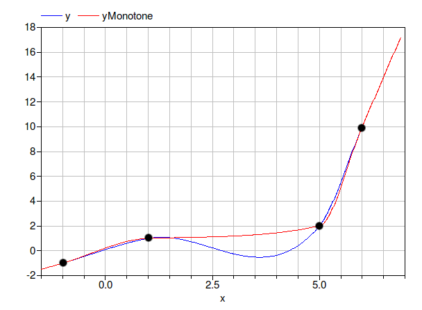
Buildings.Utilities.Math.Functions.Examples.CubicHermite

Information

This example demonstrates the use of the function for cubic hermite interpolation and linear extrapolation. The example use interpolation with two different settings: One settings produces a monotone cubic hermite, whereas the other setting does not enforce monotonicity. The resulting plot should look as shown below, where for better visibility, the support points have been marked with black dots. Notice that the red curve is monotone increasing.

Parameters

Type	Name	Default	Description
Real	xd[:]	{-1,1,5,6}	Support points
Real	yd[size(xd, 1)]	{-1,1,2,10}	Support points
Real	d[size(xd, 1)]		Derivatives at the support points
Real	dMonotone[size(xd, 1)]		Derivatives at the support points
Boolean	ensureMonotonicity	true

Modelica definition

model CubicHermite "Test problem for cubic hermite splines"
  extends Modelica.Icons.Example;
  parameter Real[:] xd={-1,1,5,6} "Support points";
  parameter Real[size(xd, 1)] yd={-1,1,2,10} "Support points";
  parameter Real[size(xd, 1)] d(each fixed=false) 
    "Derivatives at the support points";
  parameter Real[size(xd, 1)] dMonotone(each fixed=false) 
    "Derivatives at the support points";
  parameter Boolean ensureMonotonicity=true;
  Real x "Independent variable";
  Real y "Dependent variable without monotone interpolation";
  Real yMonotone "Dependent variable with monotone interpolation";
  Integer i "Integer to select data interval";
initial algorithm 
  // Get the derivative values at the support points
  d := Buildings.Utilities.Math.Functions.splineDerivatives(
    x=xd,
    y=yd,
    ensureMonotonicity=false);
  dMonotone := Buildings.Utilities.Math.Functions.splineDerivatives(x=xd, y=yd,
      ensureMonotonicity=true);
algorithm 
  x := xd[1] + time*1.2*(xd[size(xd, 1)] - xd[1]) - 0.5;
  // i is a counter that is used to pick the derivative of d or dMonotonic
  // that correspond to the interval that contains x
  i := 1;
  for j in 1:size(xd, 1) - 1 loop
    if x > xd[j] then
      i := j;
    end if;
  end for;
  // Extrapolate or interpolate the data
  y := Buildings.Utilities.Math.Functions.cubicHermiteLinearExtrapolation(
    x=x,
    x1=xd[i],
    x2=xd[i + 1],
    y1=yd[i],
    y2=yd[i + 1],
    y1d=d[i],
    y2d=d[i + 1]);
  yMonotone :=
    Buildings.Utilities.Math.Functions.cubicHermiteLinearExtrapolation(
    x=x,
    x1=xd[i],
    x2=xd[i + 1],
    y1=yd[i],
    y2=yd[i + 1],
    y1d=dMonotone[i],
    y2d=dMonotone[i + 1]);
end CubicHermite;