Modelica.Fluid.Dissipation.Utilities.Functions.General

Information

Package Content

Name	Description
CubicInterpolation_DP
CubicInterpolation_MFLOW
LambertW	Closed approximation of lambert's w function for solving f(x) = x exp(x) for x
LambertWIter	Iterative form of lambert's w function for solving f(x) = x exp(x) for x
PrandtlNumber	calculation of Prandtl number
ReynoldsNumber	calculation of Reynolds number
SmoothPower	Limiting the derivative of function y = if x>=0 then x^pow else -(-x)^pow
SmoothPower_der	The derivative of function SmoothPower
Stepsmoother	Continuous interpolation for x
Stepsmoother_der	Derivative of function Stepsmoother

Modelica.Fluid.Dissipation.Utilities.Functions.General.CubicInterpolation_DP

Inputs

Type	Name	Default	Description
Real	Re_turbulent
ReynoldsNumber	Re1		[1]
ReynoldsNumber	Re2		[1]
Real	Delta
Real	lambda2

Outputs

Type	Name	Description
ReynoldsNumber	Re	[1]

Modelica definition

function CubicInterpolation_DP
  import Modelica.Math;
  input Real Re_turbulent;
  input SI.ReynoldsNumber Re1;
  input SI.ReynoldsNumber Re2;
  input Real Delta;
  input Real lambda2;
  output SI.ReynoldsNumber Re;
  // point lg(lambda2(Re1)) with derivative at lg(Re1)
protected 
  Real x1=Math.log10(64*Re1);
  Real y1=Math.log10(Re1);
  Real yd1=1;

  // Point lg(lambda2(Re2)) with derivative at lg(Re2)
  Real aux1=(0.5/Math.log(10))*5.74*0.9;
  Real aux2=Delta/3.7 + 5.74/Re2^0.9;
  Real aux3=Math.log10(aux2);
  Real L2=0.25*(Re2/aux3)^2;
  Real aux4=2.51/sqrt(L2) + 0.27*Delta;
  Real aux5=-2*sqrt(L2)*Math.log10(aux4);
  Real x2=Math.log10(L2);
  Real y2=Math.log10(aux5);
  Real yd2=0.5 + (2.51/Math.log(10))/(aux5*aux4);

  // Constants: Cubic polynomial between lg(Re1) and lg(Re2)
  Real diff_x=x2 - x1;
  Real m=(y2 - y1)/diff_x;
  Real c2=(3*m - 2*yd1 - yd2)/diff_x;
  Real c3=(yd1 + yd2 - 2*m)/(diff_x*diff_x);
  Real lambda2_1=64*Re1;
  Real dx=Math.log10(lambda2/lambda2_1);

algorithm 
  Re := Re1*(lambda2/lambda2_1)^(1 + dx*(c2 + dx*c3));
end CubicInterpolation_DP;

Modelica.Fluid.Dissipation.Utilities.Functions.General.CubicInterpolation_MFLOW

Inputs

Type	Name	Default	Description
ReynoldsNumber	Re		[1]
ReynoldsNumber	Re1		[1]
ReynoldsNumber	Re2		[1]
Real	Delta

Outputs

Type	Name	Description
Real	lambda2

Modelica definition

function CubicInterpolation_MFLOW
  import Modelica.Math;
  input SI.ReynoldsNumber Re;
  input SI.ReynoldsNumber Re1;
  input SI.ReynoldsNumber Re2;
  input Real Delta;
  output Real lambda2;
  // point lg(lambda2(Re1)) with derivative at lg(Re1)
protected 
  Real x1=Math.log10(Re1);
  Real y1=Math.log10(64*Re1);
  Real yd1=1;

  // Point lg(lambda2(Re2)) with derivative at lg(Re2)
  Real aux1=(0.5/Math.log(10))*5.74*0.9;
  Real aux2=Delta/3.7 + 5.74/Re2^0.9;
  Real aux3=Math.log10(aux2);
  Real L2=0.25*(Re2/aux3)^2;
  Real aux4=2.51/sqrt(L2) + 0.27*Delta;
  Real aux5=-2*sqrt(L2)*Math.log10(aux4);
  Real x2=Math.log10(Re2);
  Real y2=Math.log10(L2);
  Real yd2=2 + 4*aux1/(aux2*aux3*(Re2)^0.9);

  // Constants: Cubic polynomial between lg(Re1) and lg(Re2)
  Real diff_x=x2 - x1;
  Real m=(y2 - y1)/diff_x;
  Real c2=(3*m - 2*yd1 - yd2)/diff_x;
  Real c3=(yd1 + yd2 - 2*m)/(diff_x*diff_x);
  Real dx=Math.log10(Re/Re1);

algorithm 
  lambda2 := 64*Re1*(Re/Re1)^(1 + dx*(c2 + dx*c3));
end CubicInterpolation_MFLOW;

Modelica.Fluid.Dissipation.Utilities.Functions.General.LambertW

Information

This function calculates an approximation of the inverse for

    f(x) = y = x * exp( x )

within ∞ > y > -1/e. The relative deviation of this approximation for lambert's w function x = W(y) is diplayed in the following graph.

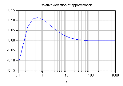
For y > 10 and higher values the relative deviation is smaller 2%.

Inputs

Type	Name	Default	Description
Real	y		f(x)

Outputs

Type	Name	Description
Real	x	W(y)

Modelica definition

function LambertW 
  "Closed approximation of lambert's w function for solving f(x) = x exp(x) for x"
  input Real y "f(x)";
  output Real x "W(y)";
protected 
  Real xl;

algorithm 
  if (y <= 500.0) then
    xl := Modelica.Math.log(y + 1.0);
    x := 0.665*(1 + 0.0195*xl)*xl + 0.04;
  else
    xl := 0;
    x := Modelica.Math.log(y - 4.0) - (1.0 - 1.0/Modelica.Math.log(y))*
      Modelica.Math.log(Modelica.Math.log(y));
  end if;

  assert(y > -1/Modelica.Math.exp(1),
    "Lambert-w-function is only valid for inputs y > -1/Modelica.Math.exp(1)!");

end LambertW;

Modelica.Fluid.Dissipation.Utilities.Functions.General.LambertWIter

Information

This function calculates an approximation of the inverse for

    f(x) = y = x * exp( x )

within ∞ > y > -1/e. Please note, that for negative inputs two solutions exists. The function currently delivers the result x = -1 ... 0 for that particular range.

Inputs

Type	Name	Default	Description
Real	y		f(x)

Outputs

Type	Name	Description
Real	x	W(y)
Integer	iter

Modelica definition

function LambertWIter 
  "Iterative form of lambert's w function for solving f(x) = x exp(x) for x"
  input Real y "f(x)";
  output Real x "W(y)";
  output Integer iter;
protected 
  Real w;
  Real prec=1e-12;
  Real c1;
  Real c2;
  Real dw;
  Real w1;
  /*Real wTimesExpW;
  Real wPlusOneTimesExpW;*/
  Real dev;
  Integer i;

algorithm 
  w := if y > 0.1 then Modelica.Fluid.Dissipation.Utilities.Functions.General.LambertW(
    y) else sqrt(5.43656*max(y, -1/Modelica.Math.exp(1)) + 2) - 1;
  dev := 1;
  i := 0;
  while prec < dev and i < 100 loop
    /*wTimesExpW := w*Modelica.Math.exp(w);
                wPlusOneTimesExpW := (w+1)*Modelica.Math.exp(w);
                w := w-(wTimesExpW-y)/(wPlusOneTimesExpW-(w+2)*(wTimesExpW-y)/(2*w+2));
                dev := abs((y-wTimesExpW)/wPlusOneTimesExpW);
                i := i+1;*/

    c1 := Modelica.Math.exp(w);
    c2 := w*c1 - y;
    w1 := if w <> 1 then w + 1 else w;
    dw := c2/(c1*w1 - ((w + 2)*c2/(2*w1)));
    w := w - dw;
    //dev := abs(dw)/(2+abs(w));
    dev := abs((y - w*c1)/(w + 1)*c1);
    i := i + 1;
  end while;
  x := w;
  iter := i;

end LambertWIter;

Modelica.Fluid.Dissipation.Utilities.Functions.General.PrandtlNumber

Inputs

Type	Name	Default	Description
SpecificHeatCapacityAtConstantPressure	cp		specific heat capacity of fluid at constant pressure [J/(kg.K)]
DynamicViscosity	eta		dynamic viscosity of fluid [Pa.s]
ThermalConductivity	lambda		thermal conductivity of fluid [W/(m.K)]

Outputs

Type	Name	Description
PrandtlNumber	Pr	Prandtl number [1]

Modelica definition

function PrandtlNumber "calculation of Prandtl number"

  import SI = Modelica.SIunits;
  import MIN = Modelica.Constants.eps;

  //fluid properties
  input SI.SpecificHeatCapacityAtConstantPressure cp 
    "specific heat capacity of fluid at constant pressure";
  input SI.DynamicViscosity eta "dynamic viscosity of fluid";
  input SI.ThermalConductivity lambda "thermal conductivity of fluid";

  output SI.PrandtlNumber Pr "Prandtl number";

algorithm 
  Pr := eta*cp/max(MIN, lambda);
end PrandtlNumber;

Modelica.Fluid.Dissipation.Utilities.Functions.General.ReynoldsNumber

Inputs

Type	Name	Default	Description
Area	A_cross		Cross sectional area [m2]
Length	perimeter		Wetted perimeter [m]
Density	rho		Density of fluid [kg/m3]
DynamicViscosity	eta		Dynamic viscosity of fluid [Pa.s]
MassFlowRate	m_flow		Mass flow rate [kg/s]

Outputs

Type	Name	Description
ReynoldsNumber	Re	Reynolds number [1]
Velocity	velocity	Mean velocity [m/s]

Modelica definition

function ReynoldsNumber "calculation of Reynolds number"

  import SI = Modelica.SIunits;
  import MIN = Modelica.Constants.eps;

  //geometry
  input SI.Area A_cross "Cross sectional area";
  input SI.Length perimeter "Wetted perimeter";

  //fluid properties
  input SI.Density rho "Density of fluid";
  input SI.DynamicViscosity eta "Dynamic viscosity of fluid";

  input SI.MassFlowRate m_flow "Mass flow rate";

  output SI.ReynoldsNumber Re "Reynolds number";
  output SI.Velocity velocity "Mean velocity";

protected 
  SI.Diameter d_hyd=4*A_cross/max(MIN, perimeter) "Hydraulic diameter";

algorithm 
  Re := 4*abs(m_flow)/max(MIN, (perimeter*eta));
  velocity := m_flow/max(MIN, (rho*A_cross));
end ReynoldsNumber;

Modelica.Fluid.Dissipation.Utilities.Functions.General.SmoothPower

Information

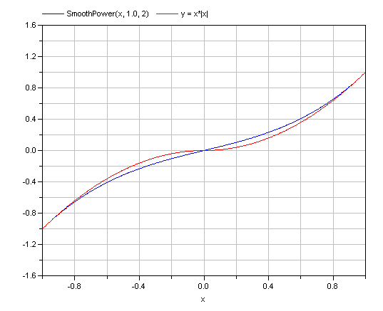
The function is used to limit the derivative of the following function at x=0:

   y = if x ≥ 0 then xpow else -(-x)pow;  // pow > 0

by approximating the function in the range -deltax< x < deltax with a third order polynomial that has the same derivative at abs(x)=deltax, as the function above.

Example

In the picture below the input x is increased from -1 to 1. The range of interpolation is defined by the same range. Displayed is the output of the function SmoothPower compared to

y=x*|x|

References

ThermoFluid Library

http://sourceforge.net/projects/thermofluid/.

Extends from Modelica.Icons.Function (Icon for functions).

Inputs

Type	Name	Default	Description
Real	x		input variable
Real	deltax		range for interpolation
Real	pow		exponent for x

Outputs

Type	Name	Description
Real	y	output variable

Modelica definition

function SmoothPower 
  "Limiting the derivative of function y = if x>=0 then x^pow else -(-x)^pow"
  annotation(derivative=SmoothPower_der);
  extends Modelica.Icons.Function;
  input Real x "input variable";
  input Real deltax "range for interpolation";
  input Real pow "exponent for x";
  output Real y "output variable";
protected 
  Real adeltax=abs(deltax);
  Real C3=(pow - 1)/2*adeltax^(pow - 3);
  Real C1=(3 - pow)/2*adeltax^(pow - 1);

algorithm 
  y := if x >= adeltax then x^pow else if x <= -adeltax then -(-x)^pow else (C1
     + C3*x*x)*x;
end SmoothPower;

Modelica.Fluid.Dissipation.Utilities.Functions.General.SmoothPower_der

Information

Inputs

Type	Name	Default	Description
Real	x		input variable
Real	deltax		range of interpolation
Real	pow		exponent for x
Real	dx		derivative of x
Real	ddeltax		derivative of deltax
Real	dpow		derivative of pow

Outputs

Type	Name	Description
Real	dy	derivative of SmoothPower

Modelica definition

function SmoothPower_der "The derivative of function SmoothPower"
  extends Modelica.Icons.Function;
  input Real x "input variable";
  input Real deltax "range of interpolation";
  input Real pow "exponent for x";
  input Real dx "derivative of x";
  input Real ddeltax "derivative of deltax";
  input Real dpow "derivative of pow";
  output Real dy "derivative of SmoothPower";
protected 
  Real C3;
  Real C1;
  Real adeltax;

algorithm 
  adeltax := abs(deltax);
  if noEvent(x >= adeltax) then
    dy := dx*pow*x^(pow - 1);
  elseif noEvent(x <= -adeltax) then
    dy := -dx*pow*(-x)^(pow - 1);
  else
    C3 := (pow - 1)/2*adeltax^(pow - 3);
    C1 := (3 - pow)/2*adeltax^(pow - 1);
    dy := (C1 + 3*C3*x*x)*dx;
  end if;
end SmoothPower_der;

Modelica.Fluid.Dissipation.Utilities.Functions.General.Stepsmoother

Information

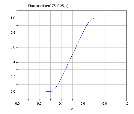
The function is used for continuous fading of variable inputs within a defined range. It allows a differentiable and smooth transition between function outputs, e.g., laminar and turbulent pressure drop or correlations for certain ranges.

Function

The tanh-function is used, since it provides an existing derivative and the derivative is zero at the borders [nofunc, func] of the interpolation domain (smooth derivative for transitions).

In order to work correctly, the internal interpolation range in terms of the external arbitrary input x needs to be scaled such that:

f(func)   = 0.5 π
f(nofunc) = -0.5 π

Example

In the picture below the input x is increased from 0 to 1. The range of interpolation is defined by:

• func = 0.75
• nofunc = 0.25

References

Wischhusen, St.

Simulation von Kältemaschinen-Prozessen mit MODELICA / DYMOLA. Diploma thesis, Hamburg University of Technology, Institute of Thermofluiddynamics, 2000.

Extends from Modelica.Icons.Function (Icon for functions).

Inputs

Type	Name	Default	Description
Real	func		input value for that result = 100%
Real	nofunc		input value for that result = 0%
Real	x		input variable for continuous interpolation

Outputs

Type	Name	Description
Real	result	output value

Modelica definition

function Stepsmoother "Continuous interpolation for x "
  annotation(derivative=Stepsmoother_der);

  extends Modelica.Icons.Function;
  input Real func "input value for that result = 100%";
  input Real nofunc "input value for that result = 0%";
  input Real x "input variable for continuous interpolation";
  output Real result "output value";

protected 
  Real m=Modelica.Constants.pi/(func - nofunc);
  Real b=-Modelica.Constants.pi/2 - m*nofunc;
  Real r_1=tan(m*x + b);

algorithm 
  result := if x >= 0.999999*(func - nofunc) + nofunc and func > nofunc or x
     <= 0.999999*(func - nofunc) + nofunc and nofunc > func then 1 else if x
     <= 0.000001*(func - nofunc) + nofunc and func > nofunc or x >= 0.000001*(
    func - nofunc) + nofunc and nofunc > func then 0 else ((0.5*(exp(r_1) - exp(
    -r_1))/(0.5*(exp(r_1) + exp(-r_1))) + 1)/2);
end Stepsmoother;

Modelica.Fluid.Dissipation.Utilities.Functions.General.Stepsmoother_der

Information

Inputs

Type	Name	Default	Description
Real	func		input for that result = 100%
Real	nofunc		input for that result = 0%
Real	x		input for interpolation
Real	dfunc		derivative of func
Real	dnofunc		derivative of nofunc
Real	dx		derivative of x

Outputs

Type	Name	Description
Real	dresult

Modelica definition

function Stepsmoother_der "Derivative of function Stepsmoother"

  extends Modelica.Icons.Function;
  input Real func "input for that result = 100%";
  input Real nofunc "input for that result = 0%";
  input Real x "input for interpolation";
  input Real dfunc "derivative of func";
  input Real dnofunc "derivative of nofunc";
  input Real dx "derivative of x";
  output Real dresult;

protected 
  Real m=Modelica.Constants.pi/(func - nofunc);
  Real b=-Modelica.Constants.pi/2 - m*nofunc;

algorithm 
  dresult := if x >= 0.999*(func - nofunc) + nofunc and func > nofunc or x <=
    0.999*(func - nofunc) + nofunc and nofunc > func or x <= 0.001*(func -
    nofunc) + nofunc and func > nofunc or x >= 0.001*(func - nofunc) + nofunc
     and nofunc > func then 0 else (1 - Modelica.Math.tanh(Modelica.Math.tan(m*
    x + b))^2)*(1 + Modelica.Math.tan(m*x + b)^2)*m*dx;
end Stepsmoother_der;