Buildings.Fluid.HeatPumps.ModularReversible.RefrigerantCycle.BaseClasses
Package with partial classes of Performance Data
Information
This package contains base classes for the package Buildings.Fluid.HeatPumps.ModularReversible.RefrigerantCycle.
Package Content
| Name | Description |
|---|---|
| Placeholder to disable heating | |
| Model with components for Carnot efficiency calculation | |
| Partial model to allow selection of only heat pump options | |
| Partial model of refrigerant cycle | |
| Partial model with components for TableData2D approach for heat pumps and chillers | |
| Calculation of capacity, heat flow rate and power based on load-dependent 2D table data | |
| Modeling block for simultaneous heating and cooling systems based on load-dependent 2D table data | |
| Collection of validation models |
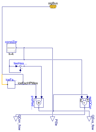
 Buildings.Fluid.HeatPumps.ModularReversible.RefrigerantCycle.BaseClasses.NoHeating
Placeholder to disable heating
Information
Using this model, the heat pump will always be off. This option is mainly used to avoid warnings about partial model which must be replaced.
Extends from PartialHeatPumpCycle (Partial model to allow selection of only heat pump options).
Parameters
| Type | Name | Default | Description |
|---|---|---|---|
| String | devIde | "NoHeating" | Indicates the data source, used to warn users about different vapor compression devices in reversible models |
| Boolean | useInHeaPum | =false to indicate that this model is used in a chiller | |
| Nominal condition | |||
| Power | PEle_nominal | 0 | Nominal electrical power consumption [W] |
| Temperature | TCon_nominal | 273.15 | Nominal temperature at secondary condenser side [K] |
| Temperature | TEva_nominal | 273.15 | Nominal temperature at secondary evaporator side [K] |
| HeatFlowRate | QHea_flow_nominal | 0 | Nominal heating capacity [W] |
| Advanced | |||
| Medium properties | |||
| SpecificHeatCapacity | cpCon | 4184 | Evaporator medium specific heat capacity [J/(kg.K)] |
| SpecificHeatCapacity | cpEva | 4184 | Evaporator medium specific heat capacity [J/(kg.K)] |
Connectors
| Type | Name | Description |
|---|---|---|
| output RealOutput | PEle | Electrical Power consumed by the device [W] |
| output RealOutput | QCon_flow | Heat flow rate through condenser [W] |
| RefrigerantMachineControlBus | sigBus | Bus-connector |
| output RealOutput | QEva_flow | Heat flow rate through evaporator [W] |
Modelica definition
Buildings.Fluid.HeatPumps.ModularReversible.RefrigerantCycle.BaseClasses.PartialCarnot
Model with components for Carnot efficiency calculation
Information
Partial model for equations and componenents used in both heat pump and chiller with the Carnot approach.
Parameters
| Type | Name | Default | Description |
|---|---|---|---|
| Boolean | useForChi | =false to use in heat pump models | |
| Nominal condition | |||
| Real | etaCarnot_nominal | 0.3 | Constant Carnot effectiveness |
| Efficiency | |||
| Boolean | use_constAppTem | false | =true to fix approach temperatures at nominal values. This can improve simulation speed |
| TemperatureDifference | TAppCon_nominal | Temperature difference between refrigerant and working fluid outlet in condenser [K] | |
| TemperatureDifference | TAppEva_nominal | Temperature difference between refrigerant and working fluid outlet in evaporator [K] | |
| Advanced | |||
| TemperatureDifference | dTCarMin | 5 | Minimal temperature difference, used to avoid division errors [K] |
Modelica definition
Buildings.Fluid.HeatPumps.ModularReversible.RefrigerantCycle.BaseClasses.PartialHeatPumpCycle
Partial model to allow selection of only heat pump options
Information
Partial refrigerant cycle model for heat pumps.
It adds the specification for frosting calculation
and restricts to the intended choices under
choicesAllMatching.
Extends from PartialRefrigerantCycle (Partial model of refrigerant cycle).
Parameters
| Type | Name | Default | Description |
|---|---|---|---|
| String | devIde | "" | Indicates the data source, used to warn users about different vapor compression devices in reversible models |
| Boolean | useInHeaPum | =false to indicate that this model is used in a chiller | |
| Nominal condition | |||
| Power | PEle_nominal | Nominal electrical power consumption [W] | |
| Temperature | TCon_nominal | Nominal temperature at secondary condenser side [K] | |
| Temperature | TEva_nominal | Nominal temperature at secondary evaporator side [K] | |
| HeatFlowRate | QHea_flow_nominal | Nominal heating capacity [W] | |
| Frosting supression | |||
| NoFrosting | iceFacCal | redeclare Buildings.Fluid.He... | Replaceable model to calculate the icing factor |
| Advanced | |||
| Medium properties | |||
| SpecificHeatCapacity | cpCon | Evaporator medium specific heat capacity [J/(kg.K)] | |
| SpecificHeatCapacity | cpEva | Evaporator medium specific heat capacity [J/(kg.K)] | |
Connectors
| Type | Name | Description |
|---|---|---|
| output RealOutput | PEle | Electrical Power consumed by the device [W] |
| output RealOutput | QCon_flow | Heat flow rate through condenser [W] |
| RefrigerantMachineControlBus | sigBus | Bus-connector |
| output RealOutput | QEva_flow | Heat flow rate through evaporator [W] |
Modelica definition
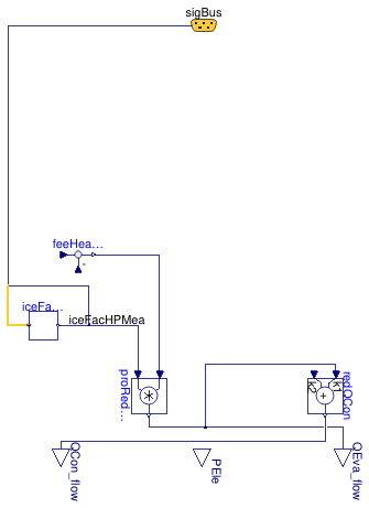
Buildings.Fluid.HeatPumps.ModularReversible.RefrigerantCycle.BaseClasses.PartialRefrigerantCycle
Partial model of refrigerant cycle
Information
Partial model for calculation of electrical power consumption
PEle, condenser heat flow QCon_flow
and evaporator heat flow QEva_flow based on the
values in the sigBus for a refrigerant machine.
Frosting performance
To simulate possible icing of the evaporator on air-source devices, the
icing factor iceFac is used to influence the outputs.
The factor models the reduction of heat transfer between refrigerant
and source. Thus, the factor is implemented as follows:
QEva_flow = iceFac * (QConNoIce_flow - PEle)
With iceFac as a relative value between 0 and 1:
iceFac = kA/kA_noIce
Finally, the energy balance must still hold:
QCon_flow = PEle + QEva_flow
You can select different options for the modeling of the icing factor or implement your own approach.
Parameters
| Type | Name | Default | Description |
|---|---|---|---|
| String | devIde | "" | Indicates the data source, used to warn users about different vapor compression devices in reversible models |
| Nominal condition | |||
| Power | PEle_nominal | Nominal electrical power consumption [W] | |
| Temperature | TCon_nominal | Nominal temperature at secondary condenser side [K] | |
| Temperature | TEva_nominal | Nominal temperature at secondary evaporator side [K] | |
| Frosting supression | |||
| NoFrosting | iceFacCal | redeclare Buildings.Fluid.He... | Replaceable model to calculate the icing factor |
| Advanced | |||
| Medium properties | |||
| SpecificHeatCapacity | cpCon | Evaporator medium specific heat capacity [J/(kg.K)] | |
| SpecificHeatCapacity | cpEva | Evaporator medium specific heat capacity [J/(kg.K)] | |
Connectors
| Type | Name | Description |
|---|---|---|
| output RealOutput | PEle | Electrical Power consumed by the device [W] |
| output RealOutput | QCon_flow | Heat flow rate through condenser [W] |
| RefrigerantMachineControlBus | sigBus | Bus-connector |
| output RealOutput | QEva_flow | Heat flow rate through evaporator [W] |
Modelica definition
Buildings.Fluid.HeatPumps.ModularReversible.RefrigerantCycle.BaseClasses.PartialTableData2D
Partial model with components for TableData2D approach for heat pumps and chillers
Information
Partial model for equations and componenents used in both heat pump and chiller models using two-dimensional data.
Parameters
| Type | Name | Default | Description |
|---|---|---|---|
| Real | scaFac | Scaling factor | |
| Boolean | use_TEvaOutForTab | true | if true, use evaporator outlet temperature, otherwise use inlet |
| Boolean | use_TConOutForTab | true | if true, use condenser outlet temperature, otherwise use inlet |
| Nominal condition | |||
| MassFlowRate | mCon_flow_nominal | Nominal mass flow rate in secondary condenser side [kg/s] | |
| MassFlowRate | mEva_flow_nominal | Nominal mass flow rate in secondary evaporator side [kg/s] | |
| Data handling | |||
| Smoothness | smoothness | Modelica.Blocks.Types.Smooth... | Smoothness of table interpolation |
| Extrapolation | extrapolation | Modelica.Blocks.Types.Extrap... | Extrapolation of data outside the definition range |
Modelica definition
 Buildings.Fluid.HeatPumps.ModularReversible.RefrigerantCycle.BaseClasses.TableData2DLoadDep
Calculation of capacity, heat flow rate and power based on load-dependent 2D table data
Information
This block implements two core features for some chiller and heat pump models within Buildings.Fluid.HeatPumps.ModularReversible and Buildings.Fluid.Chillers.ModularReversible.
-
Ideal controls: The heating or cooling load is calculated based on the block
inputs. The block returns the required part load ratio
PLRto meet the load, within system capacity.1 -
Capacity and power calculation: The capacity and power are interpolated
from user-provided data along the load side fluid temperature,
the ambient side fluid temperature
and the part load ratio
yMeaprovided as input.2
1 The part load ratio is defined as the ratio of the actual heating
(or cooling) heat flow rate to the maximum capacity of the heat pump (or chiller)
at the given load-side and ambient-side fluid temperatures.
It is dimensionless and bounded by 0 and max(PLRSup), where
the upper bound is typically equal to 1 (unless there are some
capacity margins at design conditions that need to be accounted for).
In this block, the part load ratio is used as a proxy variable
for the actual capacity modulation observable.
For systems with VFDs, this is the compressor speed.
For systems with on/off compressors, this is the capacity of the enabled
compressors divided by the total capacity.
When meeting the load by cycling on and off a single compressor,
this is the time fraction the compressor is enabled.
In all cases, the algorithm assumes continuous operation and only approximates
the performance on a time average.
Finally, note that while the part load ratio is used for generalization purposes,
either the part load ratio or the actual capacity modulation observable
(e.g., the normalized compressor speed) may be used to map the performance data.
The only requirement is that this variable be normalized, as the algorithm assumes
it equals 1 at design (selection) conditions.
2 The reason why the part load ratio is both calculated (PLR)
and exposed as an input (yMea) is to allow for modeling internal safeties
that can limit operation.
If no safeties are modeled, a direct feedback of PLR to
yMea can be used.
Capacity and power calculation
When the machine is enabled (input signal on is true)
the capacity and power are calculated by partitioning the PLR values
into three domains, as illustrated in Figure 1.
- Normal capacity modulation
This domain corresponds to the capacity range where the machine adapts to the load without false loading or cycling on and off the last operating compressor. Depending on the technology, this is achieved for example by modulating the compressor speed, throttling the inlet guide vanes or staging a varying number of compressors. In this domain, both the machine PLR and the compressor PLR vary. The capacity and power are linearly interpolated based on the performance data provided in an external file, which syntax is specified in the following section. The interpolation is carried out along three variables: the load-side fluid temperature, the ambient-side fluid temperature and the part load ratio. Note that no extrapolation is performed. The capacity and power are limited by the minimum or maximum values provided in the performance data file. - Compressor false loading
This domain corresponds to the capacity range where the machine adapts to the load by false loading the compressor. For a chiller, this is achieved by bypassing hot gas directly to the evaporator. In this domain, the machine PLR varies while the compressor PLR stays roughly the same. The input power is considered equal to the interpolated value atTLoa,TAmb,min(PLRSup). This domain may not exist if the parameterPLRCyc_minis equal tomin(PLRSup), which is the default setting. - Last operating compressor cycling
This domain corresponds to the capacity range where the last operating compressor cycles on and off. In this domain, the capacity is linearly interpolated between0and the value atTLoa,TAmb,min(PLRSup), while the power is linearly interpolated betweenP_minand the value atTLoa,TAmb,min(PLRSup), whereP_mincorresponds to the remaining power when the machine is enabled and all compressors are disabled.

Figure 1. Input power as a function of the part load ratio.
Performance data file
The performance data are read from an external ASCII file that must meet the requirements specified in the documentation of Modelica.Blocks.Tables.CombiTable2Ds.
In addition, this file must contain at least two 2D-tables that provide the maximum
heating (resp. minimum cooling) heat flow rate and the input power
of the heat pump (resp. chiller) at 100 %
PLR.
Each row of these tables corresponds to a value of the load-side
fluid temperature, each column corresponds to a value of the
ambient-side fluid temperature.
This could be either the leaving temperature if use_T*OutForTab
is true, or the entering temperature if use_T*OutForTab
is false.
The load and ambient temperatures must cover the whole operating domain,
knowing that the model only performs interpolation and no extrapolation
of the capacity and power along these variables.
The table providing the capacity values must be named q@X.XX
where X.XX is the PLR value formatted with exactly
2 decimal places ("%.2f").
Similarly, the table providing the power values must be named
p@X.XX.
Here is an example of chiller data ("-----" is not part of the file content):
-----------------------------------------------------
#1
double q@1.00(5,5)                    # Cooling heat flow rate at 100 % PLR
0 292.0 297.4 302.8 308.2             # CW temperatures as column headers
280.4 -493241 -555900 -495611 -312372 # Each row provides the capacity at a given CHW temperature
282.2 -470560 -578165 -562822 -424529
284.1 -418413 -573462 -605561 -514711
285.9 -342290 -542284 -619329 -573426
double p@1.00(5, 5)                   # Input power at 100 % PLR
0 292.0 297.4 302.8 308.2             # CW temperatures as column headers
280.4 60430 80413 80830 55530         # Each row provides the input power at a given CHW temperature
282.2 54399 80278 89151 73950
284.1 45251 76017 92822 87633
285.9 34546 68567 91833 95401
-----------------------------------------------------
In addition, for machines that have capacity modulation other than
cycling on and off a single compressor, the whole range of normal
capacity modulation must be covered by providing similar 2D-tables
at different PLR values.
The lowest PLR value will be considered as the minimum PLR value
before false loading the compressor.
If the machine has no hot gas bypass (PLRCyc_min = min(PLRSup))
this will correspond to the minimum PLR value before cycling the
last operating compressor.
All the PLR values used in the performance data file must be specified
in the array parameter PLRSup[:].
Compressor cycling
Compressor cycling is not explicitly modeled.
Instead, the model assumes continuous operation from 0 to max(PLRSup).
The only effect of cycling taken into account is the impact of the remaining power
P_min when the machine is enabled and the last operating
compressor is cycled off.
Studies on chillers and heat pumps show that this is the main driver of
efficiency loss due to cycling (Rivière, 2004).
When a compressor is staged on, energy losses occur due to the overcoming of the
refrigerant pressure equalization and the heat exchanger temperature conditioning.
However, a large part of these losses is recovered when staging off the compressor,
unless the machine is disconnected from the load when compressors are disabled.
This disconnection does not happen when staging multiple compressors,
and the research shows no significant performance degradation when a
chiller cycles between different stages without completely shutting down.
And even when disabling the last operating compressor, most plant
controls require continuous operation of the primary pumps when
the chillers or heat pumps are enabled.
The European Standard for performance rating of chillers and heat pumps
at part load conditions (CEN, 2022) states that the performance degradation due to
the pressure equalization effect when the unit restarts can be considered
as negligible for hydronic systems.
The only effect that will impact the coefficient of performance
when cycling is the remaining power input when the compressor is switching off.
If this remaining power is not measured, the Standard prescribes a default
value of 10 % of the effective power input measured
during continuous operation at part load.
Heat recovery chillers
Heat recovery chillers can be modeled with this block. In this case, the same chiller performance data file is used for both cooling and heating operation. The model assumes that all dissipated heat from the compressor is recovered by the refrigerant. This assumption enables computing the heating capacity as the sum of the cooling capacity and the input power.
When configured to represent a heat recovery chiller, this block uses an
additional input connector coo which must be true when
cooling mode is enabled, and false when heating mode is enabled.
The load side input variables must externally be connected to the
evaporator side variables in cooling mode, and to the condenser side
variables in heating mode.
The output connector Q_flow is always the
cooling heat flow rate, whatever the operating mode.
The heating heat flow rate in heating mode can be computed
externally as P-Q_flow.
Ideal controls
The block implements ideal controls by solving for the part load ratio required to meet the load (more precisely the minimum between the load and the actual capacity for the current load and ambient temperatures). This is done by interpolating the PLR values along the heat flow rate values for a given load.
The load is calculated based on the load side variables and the temperature
setpoint provided as inputs. The setpoint either represents a leaving (supply)
temperature setpoint if use_TLoaLvgForCtl is true (default setting)
or the entering (return) temperature if use_TLoaLvgForCtl is false.
The required PLR value is returned as an output while the actual heat flow rate
and power are calculated using the PLR value yMea provided as input,
which allows limiting the required PLR to account for equipment internal safeties.
References
- CEN, 2022. European Standard EN 14825:2022 E. Air conditioners, liquid chilling packages and heat pumps, with electrically driven compressors, for space heating and cooling, commercial and process cooling - Testing and rating at part load conditions and calculation of seasonal performance.
- Rivière, P. (2004). Performances saisonnières des groupes de production d’eau glaçée [Seasonal performance of liquid chillers]. École Nationale Supérieure des Mines de Paris. [In French]. https://pastel.hal.science/pastel-00001483
Extends from Modelica.Blocks.Icons.Block (Basic graphical layout of input/output block).
Parameters
| Type | Name | Default | Description |
|---|---|---|---|
| Integer | typ | ||
| Boolean | use_TLoaLvgForCtl | true | Set to true for leaving temperature control, false for entering temperature control |
| Boolean | use_TEvaOutForTab | =true to use evaporator outlet temperature for table data, false for inlet | |
| Boolean | use_TConOutForTab | =true to use condenser outlet temperature for table data, false for inlet | |
| Real | scaFac | 1 | Scaling factor for interpolated heat flow rate and power [1] |
| DimensionlessRatio | PLRSup[:] | PLR values at which heat flow rate and power data are provided [1] | |
| DimensionlessRatio | PLRCyc_min | min(PLRSup) | Minimum PLR before cycling off the last compressor [1] |
| Power | P_min | 0 | Minimum power when system is enabled with compressor cycled off [W] |
| String | fileName | File where performance data are stored | |
| Nominal condition | |||
| Temperature | TLoa_nominal | Load side fluid temperature — Entering or leaving depending on use_T*OutForTab [K] | |
| Temperature | TAmb_nominal | Ambient side fluid temperature — Entering or leaving depending on use_T*OutForTab [K] | |
| Advanced | |||
| String | tabNamQ[nPLR] | {"q@" + String(p, format=".2... | Table names with heat flow rate data |
| String | tabNamP[nPLR] | {"p@" + String(p, format=".2... | Table names with power data |
Connectors
| Type | Name | Description |
|---|---|---|
| input BooleanInput | on | Set to true to enable compressor, or false to disable compressor |
| input BooleanInput | coo | Switchover signal: true for cooling, false for heating |
| input RealInput | TLoaEnt | Entering fluid temperature on load side [K] |
| input RealInput | TAmbEnt | Entering fluid temperature on ambient side [K] |
| input RealInput | TSet | Temperature setpoint [K] |
| input RealInput | TLoaLvg | Leaving fluid temperature on load side [K] |
| input RealInput | mLoa_flow | Fluid mass flow rate on load side [kg/s] |
| output RealOutput | P | Input power [W] |
| output RealOutput | PLR | Compressor part load ratio to meet the load (within capacity) [1] |
| output RealOutput | Q_flow | Heat flow rate [J/s] |
| input RealInput | TAmbLvg | Leaving fluid temperature on ambient side [K] |
| input RealInput | yMea | Capacity limiting signal yielded by internal safety logic [1] |
| input RealInput | cpLoa | Specific heat capacity of fluid on load side [J/(kg.K)] |
Modelica definition
 Buildings.Fluid.HeatPumps.ModularReversible.RefrigerantCycle.BaseClasses.TableData2DLoadDepSHC
Modeling block for simultaneous heating and cooling systems based on load-dependent 2D table data

Information
This block provides the core implementation to model simultaneous heating and
cooling (SHC) systems, also referred to as multipipe polyvalent units or "Type A"
in Eurovent (2025).
Since the most recent versions of these systems are composed of multiple modules,
the implementation includes the staging logic for an arbitrary number of
modules nUni. Nevertheless, single-module systems can also be
appropriately represented by setting nUni = 1.
All kinds of capacity-modulation processes are supported, such as VFD-driven compressors, multiple on-off compressors, and single compressor cycling. The method used to interpolate capacity and power based on user-provided data is taken from Buildings.Fluid.HeatPumps.ModularReversible.RefrigerantCycle.BaseClasses.TableData2DLoadDep. Users should be familiar with this latter block before continuing with this documentation.
The block implements the following functionalities:
- Ideal controls.
- Capacity and power calculation.
- Module staging.
- Load balancing between the HW and CHW side.
System and module operating mode
The block inputs onHea and onCoo allow switching between
three system operating modes.
- Heating-only: In this mode, all modules operate as heat pumps, tracking the HW temperature setpoint and sourcing heat from the ambient-side fluid.
- Cooling-only: In this mode, all modules operate as chillers, tracking the CHW temperature setpoint and rejecting heat to the ambient-side fluid.
- Simultaneous heating and cooling: In this mode, some modules operate as heat recovery chillers, sourcing heat from the CHW circuit and rejecting heat to the HW circuit. The system load balancing logic (see Section "Load balancing between the HW and CHW side") ensures that, on average, both the HW temperature setpoint and the CHW temperature setpoint are met by these modules. Additional modules may concurrently run in heating-only or cooling-only mode to match the residual load. In the extreme case where the system is only exposed to heating (resp. cooling) loads, all modules will run in heating-only (resp. cooling-only) mode.
Ideal controls
For each module operating mode, the block implements ideal controls by solving for the part load ratio required to meet the load (more precisely the minimum between the load and the actual capacity for the current source and sink temperatures). This is done by interpolating the PLR values along the heat flow rate values for a given load. As described in Section "Load balancing between the HW and CHW side", the part load ratio for modules in SHC mode is the maximum between the PLR values for the heating load and the cooling load.
The load is calculated based on the HW and CHW-side side variables and the temperature setpoint
provided as inputs. The setpoint either represents a leaving (supply) temperature setpoint if
use_TLoaLvgForCtl is true (default setting) or the entering (return)
temperature if use_TLoaLvgForCtl is false.
In contrast to the implementation in Buildings.Fluid.HeatPumps.ModularReversible.RefrigerantCycle.BaseClasses.TableData2DLoadDep the current block does not expose the PLR value, and therefore does not support external modeling of equipment safeties.
Capacity and power calculation
The capacity and power calculation follows the same logic as the one described in
Buildings.Fluid.HeatPumps.ModularReversible.RefrigerantCycle.BaseClasses.TableData2DLoadDep
except that the current block does not include compressor false loading, i.e., both the capacity
and power are linearly interpolated along PLR between 0 and min(PLR<Shc|Hea|Coo>Sup).
Performance data file and scaling
The performance data are read from external ASCII files that must meet the requirements specified in the documentation of Buildings.Fluid.HeatPumps.ModularReversible.RefrigerantCycle.BaseClasses.TableData2DLoadDep.
A performance data file must be provided for each module operating mode:
heating-only, cooling-only and simultaneous heating and cooling.
It is expected that performance data be provided for a single module.
This is however a loose requirement as the scaling logic anyway ensures that
the nominal heat flow rates Q*_flow_nominal provided as parameters
match the values interpolated from the performance data, times the number of modules.
Note that for single-mode performance data, the ambient-side fluid temperature
must correspond to the entering temperature, while the model supports
choosing between entering or leaving temperature for the CHW and HW via
the parameters use_TEvaOutForTab and use_TConOutForTab,
respectively.
Module staging
First, the heating and cooling loads QHeaSet_flow and QCooSet_flow
are calculated from the block inputs (see Section "Ideal controls").
The staging logic uses time-averaged heating and cooling loads
QHeaSetMea_flow and QCooSetMea_flow.
An exponential moving average (dtMea * der(Q<Hea|Coo>SetMea_flow) =
Q<Hea|Coo>Set_flow - Q<Hea|Coo>SetMea_flow)
is used for computational efficiency.
Then the model evaluates the capacity of a single module in each mode, based on the current source and sink fluid temperature (see Section "Capacity and power calculation"). The number of modules required to run to meet the load is then calculated for each mode as follows.
-
Number of modules required to run in SHC mode to meet the heating load as
nUniHeaShcRaw = ceil(QHeaSetMea_flow / max(QHeaShcInt_flow) / SPLR),
wheremax(QHeaShcInt_flow)is the heating capacity of one module in SHC mode andSPLRis a parameter representing the staging part load ratio. Note that this parameter should be strictly lower than1because the number of staged modules ultimately conditions the opening of isolation valves and the staging of primary pumps. IfSPLR = 1it is likely that the mass flow rate will limit the load below the capacity of a single module, practically preventing the system from staging up until the return temperature exceeds the design value. -
Number of modules required to run in SHC mode to meet the cooling load as
nUniCooShcRaw = ceil(QCooSetMea_flow / min(QCooSHcInt_flow) / SPLR),
wheremin(QCooSHcInt_flow)is the cooling capacity of one module in SHC mode. -
Number of modules required to run in SHC mode as
nUniShcRaw = min(nUniCooShcRaw, nUniHeaShcRaw).
This condition means that the system stops staging modules in SHC mode when either the cooling load or the heating load is met. -
Number of modules required to run in heating mode as
nUniHeaRaw = ceil(QHeaSetResMea_flow / max(QHeaInt_flow) / SPLR),
whereQHeaSetResMea_flowis the residual heating load, calculated as the time-averaged heating load minus the heating output of modules in SHC mode, andmax(QHeaInt_flow)is the capacity of one module in heating-only mode. -
Number of modules required to run in cooling mode as
nUniCooRaw = ceil(QCooSetResMea_flow / min(QCooInt_flow) / SPLR),
whereQCooSetResMea_flowis the residual cooling load, calculated as the time-averaged cooling load minus the cooling output of modules in SHC mode, andmin(QCooInt_flow)is the capacity of one module in cooling-only mode.
Discrete-event logic is then used to calculate the actual number of modules in
each mode (nUniShc, nUniHea and nUniCoo)
considering the following requirements.
- Minimum stage runtime: The number of modules enabled in each mode must stay unchanged
for at least
dtRun. - Step-by-step staging: Only one module can be enabled or disabled on the HW side at the same time, and similarly for the CHW side. However, "hot swapping" is allowed, where one module can be enabled or disabled in SHC mode while one module is simultaneously being disabled or enabled in heating or cooling mode.
- Priority order: When the total number of modules required to run in each mode
(
nUniShcRaw + nUniHeaRaw + nUniCooRaw) exceeds the number of modules in the bank, the following priority applies where modules required in SHC mode are staged first and modules required in cooling mode are staged last.
Load balancing between the HW and CHW side
A fundamental assumption for load balancing is that the system is composed of equally sized modules that are hydronically balanced, connected in parallel arrangement and controlled at the same setpoint. This implies that each module connected to the HW (resp. CHW) loop handles an equal fraction of the total heating (resp. cooling) load, irrespective of whether the module operates in SHC or single mode. This assumption is strictly true on the dominant side. However, as explained below, it is only partially true on the non-dominant side where setpoint deviations occur in the modules with excess thermal output and in the compensating module.
Based on this assumption, on the dominant side, the heating or cooling load of each module in SHC mode can be calculated as
Q<Hea|Coo>SetUniShc_flow = Q<Hea|Coo>Set_flow / (nUniShc + nUni<Hea|Coo>).
In order to achieve load balancing between the CHW and HW sides for the subset of modules in SHC mode, the model assumes that these modules are loaded for the most demanding side, and that a single module can cycle between SHC and the corresponding single-mode operation. For example, in case of 90 % cooling load and 60 % heating load, the module will cycle between SHC at 90 % PLR during 2/3 of the time and cooling-only at 90 % PLR during 1/3 of the time. This logic is inspired from the sequence of operation of a multipipe heat pump system (Johnson Controls, 2024) where the last enabled circuit cycles between SHC and single-mode operation to balance the heating and cooling loads.
The part load ratio of each module in SHC mode to satisfy the most demanding side is
PLRShcLoa = min(PLRShcSup, max(fHeaShc-1(QHeaSetUniShc_flow),
fCooShc-1(QCooSetUniShc_flow)))
,
where f<Hea|Coo>Shc-1 is the linear interpolation of the part
load ratio along the module heating or cooling capacity at the actual source and sink temperature,
based on the performance data provided for SHC operation.
A demand limiting logic is implemented to prevent overcooling or overheating due to the stage
minimum runtime requirement and the possible flow variations resulting from modulating the primary
pump speed and/or the minimum flow bypass valve.
This logic uses a temperature deviation from setpoint dTSaf, which is converted to
limiting heat flow rates Q<Hea|Coo>Saf_flow.
The limiting part load ratio is calculated as
PLRShcSaf = min(fHeaShc-1(QHeaSaf_flow / (nUniShc + nUniHea)),
fCooShc-1(QCooSaf_flow / (nUniShc + nUniCoo)))
.
The effective part load ratio of each module in SHC mode is then the minimum of the load-based and safety-limited values
PLRShc = min(PLRShcLoa, PLRShcSaf).
The excess heating or cooling heat flow rate (non-dominant side) of the modules in SHC mode is then calculated as
Q<Hea|Coo>ShcExc_flow = nUniShc * (f<Hea|Coo>Shc(PLRShc) -
Q<Hea|Coo>SetUniShc_flow)
,
where f<Hea|Coo>Shc is the linear interpolation of the module heating or
cooling capacity along the part load ratio at the actual source and sink temperature,
based on the performance data provided for SHC operation.
This excess heat flow rate is compensated by cycling a single module, which gives theg expression of the cycling ratio for this module as
ratCycShc = 1 - min(1, max(QHeaShcExc_flow / fHeaShc(PLRShc), QCooShcExc_flow / fCooShc(PLRShc))),
where ratCycShc = 1 means perfect balance, i.e., the module does not cycle and
continuously runs in SHC mode, and ratCycShc = 0 means that the module continuously
runs in single mode.
The actual heating or cooling heat flow rate of the modules in SHC mode is
Q<Hea|Coo>Shc_flow = (nUniShc - 1 + ratCycShc) * f<Hea|Coo>Shc(PLRShc).
The residual load that the module which cycles between SHC and single-mode must handle is
Q<Hea|Coo>SetUniShc_flow * nUniShc - Q<Hea|Coo>Shc_flow,
which gives the part load ratio PLR<Hea|Coo>ShcCyc of this module while
it runs in single mode.
The corresponding heating or cooling heat flow rate is then
Q<Hea|Coo>ShcCyc_flow = (1 - ratCycShc) * f<Hea|Coo>(PLR<Hea|Coo>ShcCyc),
where f<Hea|Coo> is the linear interpolation of the module capacity along
the part load ratio at the actual source and sink temperature,
based on the performance data provided for single-mode operation.
The residual heating or cooling loads that the modules running in single mode must meet can now be calculated as
Q<Hea|Coo>SetRes_flow = Q<Hea|Coo>Set_flow -
(Q<Hea|Coo>Shc_flow + Q<Hea|Coo>ShcCyc_flow)
,
which ultimately allows calculating the PLR value of these modules and their contribution to the total heating and cooling output of the bank.
Implementation limitations
The load balancing logic relies on a subset of modules producing excess heat flow rate
while another module compensates for it.
The fundamental assumption of even load between modules therefore breaks down on
the non-dominant side.
In a real system where the modules are hydronically balanced, this load imbalance yields
varying leaving temperatures across modules.
In the worst case, the deviation from setpoint is ΔT⋅SPLR / 2,
where ΔT is the design temperature difference.
These temperature discrepancies are neglected in the model which "numerically absorbs" them by simply adjusting the load that each module must handle. This creates a modeling uncertainty that is deemed acceptable given the error magnitude and partial cancellation of opposing errors from modules that exhibit setpoint overshoot and modules that exhibit setpoint undershoot.
References
- Eurovent (2025). Technical certification rules (TCR) of the Eurovent certified performance mark liquid chilling packages and hydronic heat pumps (ECP - 3 LCPHP, Rev. 02-2025). https://www.eurovent-certification.com/media/images/c2c/031/c2c031f2dd38173a81e30a42f7d6f42a386f047c.pdf
- Johnson Controls, Inc. (2024). YMAE application guide - YMAE air-to-water inverter scroll heat pumps. YORK.
Parameters
| Type | Name | Default | Description |
|---|---|---|---|
| Integer | nUni | 1 | Number of modules |
| Boolean | use_TLoaLvgForCtl | true | Set to true for leaving temperature control, false for entering temperature control |
| Boolean | use_TEvaOutForTab | =true to use CHW temperature at outlet for table data, false for inlet | |
| Boolean | use_TConOutForTab | =true to use HW temperature at outlet for table data, false for inlet | |
| DimensionlessRatio | PLRHeaSup[:] | PLR values at which heat flow rate and power data are provided - Heating [1] | |
| DimensionlessRatio | PLRCooSup[:] | PLR values at which heat flow rate and power data are provided - Cooling [1] | |
| DimensionlessRatio | PLRShcSup[:] | PLR values at which heat flow rate and power data are provided - SHC [1] | |
| Power | P_min | 0 | Remaining power when system is enabled with all compressors cycled off [W] |
| String | fileNameHea | File where performance data are stored - Heating (single module) | |
| String | fileNameCoo | File where performance data are stored - Cooling (single module) | |
| String | fileNameShc | File where performance data are stored - SHC (single module) | |
| Nominal condition | |||
| Temperature | THw_nominal | HW temperature — Entering or leaving depending on use_TConOutForTab [K] | |
| Temperature | TChw_nominal | CHW temperature — Entering or leaving depending on use_TEvaOutForTab [K] | |
| Nominal condition - Heating | |||
| Temperature | TAmbHea_nominal | Ambient-side fluid temperature — Entering [K] | |
| HeatFlowRate | QHea_flow_nominal | Heating heat flow rate - All modules [W] | |
| Nominal condition - Cooling | |||
| Temperature | TAmbCoo_nominal | Ambient-side fluid temperature — Entering [K] | |
| HeatFlowRate | QCoo_flow_nominal | Cooling heat flow rate - All modules [W] | |
| Nominal condition - SHC | |||
| HeatFlowRate | QHeaShc_flow_nominal | Heating heat flow rate - All modules [W] | |
| HeatFlowRate | QCooShc_flow_nominal | Cooling heat flow rate - All modules [W] | |
| Advanced | |||
| String | tabNamQHea[nPLRHea] | {"q@" + String(p, format=".2... | Table names with heat flow rate data - Heating |
| String | tabNamPHea[nPLRHea] | {"p@" + String(p, format=".2... | Table names with power data - Heating |
| String | tabNamQCoo[nPLRCoo] | {"q@" + String(p, format=".2... | Table names with heat flow rate data - Cooling |
| String | tabNamPCoo[nPLRCoo] | {"p@" + String(p, format=".2... | Table names with power data - Cooling |
| String | tabNamQShc[nPLRShc] | {"q@" + String(p, format=".2... | Table names with cooling heat flow rate data - SHC |
| String | tabNamPShc[nPLRShc] | {"p@" + String(p, format=".2... | Table names with power data - SHC |
| Staging logic | |||
| Real | dtRun | 300 | Minimum stage runtime [s] |
| Real | dtMea | 120 | Load averaging time window [s] |
| Real | SPLR | 0.9 | Staging part load ratio |
| Safeties | |||
| TemperatureDifference | dTSaf | 2 | Maximum temperature deviation from setpoint before limiting demand for safety (>0) [K] |
Connectors
| Type | Name | Description |
|---|---|---|
| input BooleanInput | onHea | Heating on/off command |
| input BooleanInput | onCoo | Cooling on/off command |
| input RealInput | THwEnt | Condenser entering HW temperature [K] |
| input RealInput | THwLvg | Condenser leaving HW temperature [K] |
| input RealInput | TChwEnt | Evaporator entering CHW temperature [K] |
| input RealInput | TChwLvg | Evaporator leaving CHW temperature [K] |
| input RealInput | TAmbEnt | Entering fluid temperature on ambient side [K] |
| input RealInput | cpHw | HW specific heat capacity [J/(kg.K)] |
| input RealInput | cpChw | CHW specific heat capacity [J/(kg.K)] |
| input RealInput | TChwSet | CHW temperature setpoint [K] |
| input RealInput | THwSet | HW temperature setpoint [K] |
| input RealInput | mHw_flow | HW mass flow rate [kg/s] |
| input RealInput | mChw_flow | CHW mass flow rate [kg/s] |
| output RealOutput | P | Input power [W] |
| output RealOutput | QHea_flow | Heating heat flow rate [J/s] |
| output RealOutput | QCoo_flow | Cooling heat flow rate [J/s] |
| output IntegerOutput | nUniHea | Number of modules in heating mode |
| output IntegerOutput | nUniCoo | Number of modules in cooling mode |
| output IntegerOutput | nUniShc | Number of modules in SHC mode (may be cycling into single mode) |