Buildings.Fluid.Chillers
Package with models for chillers
Information
This package contains component models for chillers.
For heat pump models, see Buildings.Fluid.HeatPumps.
Extends from Modelica.Icons.Package (Icon for standard packages).
Package Content
| Name | Description |
|---|---|
| Indirect steam heated absorption chiller based on performance curves | |
| Chiller with prescribed evaporator leaving temperature and performance curve adjusted based on Carnot efficiency | |
| Chiller with performance curve adjusted based on Carnot efficiency | |
| Electric chiller based on the DOE-2.1 model | |
| Electric chiller based on the DOE-2.1 model, but with performance as a function of condenser leaving instead of entering temperature | |
| Package for reversible and non-reversible chillers using a modular model approach | |
| Performance data for electric chillers | |
| Collection of models that illustrate model use and test models | |
| Collection of models that validate the chiller models | |
| Package with base classes for Buildings.Fluid.Chillers |
 Buildings.Fluid.Chillers.AbsorptionIndirectSteam
Indirect steam heated absorption chiller based on performance curves
Information
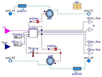
Model for an indirect steam heated absorption chiller based on performance curves.
The model uses performance curves similar to the EnergyPlus model Chiller:Absorption:Indirect.
The model uses six functions to predict the chiller cooling capacity, power consumption for
the chiller pump and the generator heat flow rate and the condenser heat flow.
These functions use the performance data stored in the record per.
The computations are as follows:
The capacity function of the evaporator is
capFuneva = A1 + A2 Teva,lvg + A3 T2eva,lvg + A4 T3eva,lvg.
The capacity function of the condenser is
capFuncon = B1 + B2 Tcon,ent + B3 T2con,ent + B4 T3con,ent.
These capacity functions are used to compute the available cooling capacity of the evaporator as
Q̇eva,ava = capFuneva capFuncon Q̇eva,0,
where Q̇eva,0 is obtained from the performance data per.QEva_flow_nominal.
Let Q̇eva,set denote the heat required to meet the set point TSet.
Then, the model computes the part load ratio as
PLR =min(Q̇eva,set/Q̇eva,ava, PLRmax).
Hence, the model ensures that the chiller capacity does not exceed the chiller capacity specified
by the parameter per.PLRMax.
The cycling ratio is computed as
CR = min(PLR/PLRmin, 1.0),
where PRLmin is obtained from the performance record per.PLRMin.
This ratio expresses the fraction of time
that a chiller would run if it were to cycle because its load is smaller than the
minimal load at which it can operate.
Note that this model continuously operates even if the part load ratio is below the
minimum part load ratio.
Its leaving evaporator and condenser temperature can therefore be considered as an
average temperature between the modes when the compressor is off and on.
Using the part load ratio, the energy input ratio of the chiller pump is
EIRP = C1 + C2PLR+C3PLR2.
The generator heat input ratio is
genHIR = D1 + D2PLR+D3PLR2+D4PLR3.
Two additional curves modify the heat input requirement based on the condenser inlet water temperature and the evaporator outlet water temperature. Specifically, the generator heat modifier based on the condenser inlet water temperature is
genTcon = E1 + E2 Tcon,ent + E3 T2con,ent + E4 T3con,ent,
and the generator heat modifier based on the evaporator inlet water temperature is
genTeva= F1 + F2 Teva,lvg + F3 T2eva,lvg + F4 T3eva,lvg.
The main outputs of the model that are to be used in energy analysis
are the required generator heat QGen_flow and
the electric power consumption of the chiller pump P.
For example, if the chiller were to be regenerated with steam, then
QGen_flow is the heat that must be provided by a steam loop.
This model computes the required generator heat as
Q̇gen = -Q̇eva,ava genHIR genTcon genTeva CR.
The pump power consumption is
P = EIRP CR P0,
where P0 is the pump nominal power obtained from the performance data per.P_nominal.
The heat balance of the chiller is
Q̇con = -Q̇eva + Q̇gen + P.
Performance data
The equipment performance data is obtained from the record per,
which is an instance of
Buildings.Fluid.Chillers.Data.AbsorptionIndirectSteam.
Additional performance curves can be developed using
two available techniques (Hydeman and Gillespie, 2002). The first technique is called the
Least-squares Linear Regression method and is used when sufficient performance data exist
to employ standard least-square linear regression techniques. The second technique is called
Reference Curve Method and is used when insufficient performance data exist to apply linear
regression techniques. A detailed description of both techniques can be found in
Hydeman and Gillespie (2002).
References
- Hydeman, M. and K.L. Gillespie. 2002. Tools and Techniques to Calibrate Electric Chiller Component Models. ASHRAE Transactions, AC-02-9-1.
Extends from Buildings.Fluid.Interfaces.FourPortHeatMassExchanger (Model transporting two fluid streams between four ports with storing mass or energy).
Parameters
| Type | Name | Default | Description |
|---|---|---|---|
| replaceable package Medium1 | PartialMedium | Medium 1 in the component | |
| replaceable package Medium2 | PartialMedium | Medium 2 in the component | |
| Generic | per | Performance data | |
| Nominal condition | |||
| MassFlowRate | m1_flow_nominal | per.mCon_flow_nominal | Nominal mass flow rate [kg/s] |
| MassFlowRate | m2_flow_nominal | per.mEva_flow_nominal | Nominal mass flow rate [kg/s] |
| PressureDifference | dp1_nominal | per.dpCon_nominal | Pressure difference [Pa] |
| PressureDifference | dp2_nominal | per.dpEva_nominal | Pressure difference [Pa] |
| Assumptions | |||
| Boolean | allowFlowReversal1 | true | = false to simplify equations, assuming, but not enforcing, no flow reversal for medium 1 |
| Boolean | allowFlowReversal2 | true | = false to simplify equations, assuming, but not enforcing, no flow reversal for medium 2 |
| Advanced | |||
| MassFlowRate | m1_flow_small | 1E-4*abs(m1_flow_nominal) | Small mass flow rate for regularization of zero flow [kg/s] |
| MassFlowRate | m2_flow_small | 1E-4*abs(m2_flow_nominal) | Small mass flow rate for regularization of zero flow [kg/s] |
| HeatFlowRate | Q_flow_small | -per.QEva_flow_nominal*1E-6 | Small value for heat flow rate or power, used to avoid division by zero [W] |
| Diagnostics | |||
| Boolean | show_T | false | = true, if actual temperature at port is computed |
| Flow resistance | |||
| Medium 1 | |||
| Boolean | from_dp1 | false | = true, use m_flow = f(dp) else dp = f(m_flow) |
| Boolean | linearizeFlowResistance1 | false | = true, use linear relation between m_flow and dp for any flow rate |
| Real | deltaM1 | 0.1 | Fraction of nominal flow rate where flow transitions to laminar |
| Medium 2 | |||
| Boolean | from_dp2 | false | = true, use m_flow = f(dp) else dp = f(m_flow) |
| Boolean | linearizeFlowResistance2 | false | = true, use linear relation between m_flow and dp for any flow rate |
| Real | deltaM2 | 0.1 | Fraction of nominal flow rate where flow transitions to laminar |
| Dynamics | |||
| Nominal condition | |||
| Time | tau1 | 30 | Time constant at nominal flow [s] |
| Time | tau2 | 30 | Time constant at nominal flow [s] |
| Conservation equations | |||
| Dynamics | energyDynamics | Modelica.Fluid.Types.Dynamic... | Type of energy balance: dynamic (3 initialization options) or steady state |
| Initialization | |||
| Medium 1 | |||
| AbsolutePressure | p1_start | Medium1.p_default | Start value of pressure [Pa] |
| Temperature | T1_start | 273.15 + 25 | Start value of temperature [K] |
| MassFraction | X1_start[Medium1.nX] | Medium1.X_default | Start value of mass fractions m_i/m [kg/kg] |
| ExtraProperty | C1_start[Medium1.nC] | fill(0, Medium1.nC) | Start value of trace substances |
| ExtraProperty | C1_nominal[Medium1.nC] | fill(1E-2, Medium1.nC) | Nominal value of trace substances. (Set to typical order of magnitude.) |
| Medium 2 | |||
| AbsolutePressure | p2_start | Medium2.p_default | Start value of pressure [Pa] |
| Temperature | T2_start | 273.15 + 5 | Start value of temperature [K] |
| MassFraction | X2_start[Medium2.nX] | Medium2.X_default | Start value of mass fractions m_i/m [kg/kg] |
| ExtraProperty | C2_start[Medium2.nC] | fill(0, Medium2.nC) | Start value of trace substances |
| ExtraProperty | C2_nominal[Medium2.nC] | fill(1E-2, Medium2.nC) | Nominal value of trace substances. (Set to typical order of magnitude.) |
Connectors
| Type | Name | Description |
|---|---|---|
| FluidPort_a | port_a1 | Fluid connector a1 (positive design flow direction is from port_a1 to port_b1) |
| FluidPort_b | port_b1 | Fluid connector b1 (positive design flow direction is from port_a1 to port_b1) |
| FluidPort_a | port_a2 | Fluid connector a2 (positive design flow direction is from port_a2 to port_b2) |
| FluidPort_b | port_b2 | Fluid connector b2 (positive design flow direction is from port_a2 to port_b2) |
| input BooleanInput | on | Set to true to enable the absorption chiller |
| input RealInput | TSet | Evaporator setpoint leaving water temperature [K] |
| output RealOutput | P | Chiller pump power [W] |
| output RealOutput | QGen_flow | Required generator heat flow rate in the form of steam [W] |
| output RealOutput | QEva_flow | Evaporator heat flow rate [W] |
| output RealOutput | QCon_flow | Condenser heat flow rate [W] |
Modelica definition
 Buildings.Fluid.Chillers.Carnot_TEva
Chiller with prescribed evaporator leaving temperature and performance curve adjusted based on Carnot efficiency
Information
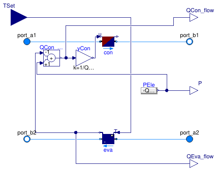
This is a model of a chiller whose coefficient of performance COP changes with temperatures in the same way as the Carnot efficiency changes. The control input is the setpoint of the evaporator leaving temperature, which is met exactly at steady state if the chiller has sufficient capacity.
Set use_eta_Carnot_nominal=true to specify directly
the Carnot effectiveness ηCarnot,0,
in which case the value of the parameter COP_nominal
will not affect the simulation.
If use_eta_Carnot_nominal=false, the model will use
the value of the parameter COP_nominal
together with the specified nominal temperatures
to compute the Carnot effectiveness as
ηCarnot,0 = COP0 ⁄ (Teva,0 ⁄ (Tcon,0 + Tapp,con,0 - (Teva,0-Tapp,eva,0))),
where Teva,0 is the evaporator temperature, Tcon,0 is the condenser temperature, Tapp,eva,0 is the evaporator approach temperature and Tapp,con,0 is the condenser approach temperature.
The COP is computed as the product
COP = ηCarnot,0 COPCarnot ηPL,
where COPCarnot is the Carnot efficiency and ηPL is the part load efficiency, expressed using a polynomial. This polynomial has the form
ηPL = a1 + a2 y + a3 y2 + ...,
where y ∈ [0, 1] is
the part load for cooling and the coefficients ai
are declared by the parameter a.
On the Dynamics tag, the model can be parametrized to compute a transient
or steady-state response.
The transient response of the model is computed using a first
order differential equation for the evaporator and condenser fluid volumes.
The chiller outlet temperatures are equal to the temperatures of these lumped volumes.
Typical use and important parameters
When using this component, make sure that the condenser has sufficient mass flow rate. Based on the evaporator mass flow rate, temperature difference and the efficiencies, the model computes how much heat will be added to the condenser. If the mass flow rate is too small, very high outlet temperatures can result.
The evaporator heat flow rate QEva_flow_nominal is used to assign
the default value for the mass flow rates, which are used for the pressure drop
calculations.
It is also used to compute the part load efficiency.
Hence, make sure that QEva_flow_nominal is set to a reasonable value.
The maximum cooling capacity is set by the parameter QEva_flow_min,
which is by default set to negative infinity.
The coefficient of performance depends on the evaporator and condenser leaving temperature since otherwise the second law of thermodynamics may be violated.
Notes
For a similar model that can be used as a heat pump, see Buildings.Fluid.HeatPumps.Examples.Carnot_TCon.
Extends from Buildings.Fluid.Chillers.BaseClasses.PartialCarnot_T (Partial model for chiller with performance curve adjusted based on Carnot efficiency).
Parameters
| Type | Name | Default | Description |
|---|---|---|---|
| replaceable package Medium1 | PartialMedium | Medium 1 in the component | |
| replaceable package Medium2 | PartialMedium | Medium 2 in the component | |
| HeatFlowRate | QEva_flow_min | -Modelica.Constants.inf | Maximum heat flow rate for cooling (negative) [W] |
| Nominal condition | |||
| MassFlowRate | m1_flow_nominal | QCon_flow_nominal/cp1_defaul... | Nominal mass flow rate [kg/s] |
| MassFlowRate | m2_flow_nominal | QEva_flow_nominal/cp2_defaul... | Nominal mass flow rate [kg/s] |
| HeatFlowRate | QEva_flow_nominal | Nominal cooling heat flow rate (QEva_flow_nominal < 0) [W] | |
| HeatFlowRate | QCon_flow_nominal | -QEva_flow_nominal*(1 + COP_... | Nominal heating flow rate [W] |
| TemperatureDifference | dTEva_nominal | -10 | Temperature difference evaporator outlet-inlet [K] |
| TemperatureDifference | dTCon_nominal | 10 | Temperature difference condenser outlet-inlet [K] |
| Pressure | dp1_nominal | Pressure difference over condenser [Pa] | |
| Pressure | dp2_nominal | Pressure difference over evaporator [Pa] | |
| Efficiency | |||
| Boolean | use_eta_Carnot_nominal | true | Set to true to use Carnot effectiveness etaCarnot_nominal rather than COP_nominal |
| Real | etaCarnot_nominal | 0.3 | Carnot effectiveness (=COP/COP_Carnot) used during simulation if use_eta_Carnot_nominal = true [1] |
| Real | COP_nominal | etaCarnot_nominal*TUseAct_no... | Coefficient of performance at TEva_nominal and TCon_nominal, used during simulation if use_eta_Carnot_nominal = false [1] |
| Temperature | TCon_nominal | 303.15 | Condenser temperature used to compute COP_nominal if use_eta_Carnot_nominal=false [K] |
| Temperature | TEva_nominal | 278.15 | Evaporator temperature used to compute COP_nominal if use_eta_Carnot_nominal=false [K] |
| Real | a[:] | {1} | Coefficients for efficiency curve (need p(a=a, yPL=1)=1) |
| TemperatureDifference | TAppCon_nominal | if cp1_default < 1500 then 5... | Temperature difference between refrigerant and working fluid outlet in condenser [K] |
| TemperatureDifference | TAppEva_nominal | if cp2_default < 1500 then 5... | Temperature difference between refrigerant and working fluid outlet in evaporator [K] |
| Assumptions | |||
| Boolean | allowFlowReversal1 | true | = false to simplify equations, assuming, but not enforcing, no flow reversal for medium 1 |
| Boolean | allowFlowReversal2 | true | = false to simplify equations, assuming, but not enforcing, no flow reversal for medium 2 |
| Advanced | |||
| MassFlowRate | m1_flow_small | 1E-4*abs(m1_flow_nominal) | Small mass flow rate for regularization of zero flow [kg/s] |
| MassFlowRate | m2_flow_small | 1E-4*abs(m2_flow_nominal) | Small mass flow rate for regularization of zero flow [kg/s] |
| Diagnostics | |||
| Boolean | show_T | false | = true, if actual temperature at port is computed |
| Flow resistance | |||
| Condenser | |||
| Boolean | from_dp1 | false | = true, use m_flow = f(dp) else dp = f(m_flow) |
| Boolean | linearizeFlowResistance1 | false | = true, use linear relation between m_flow and dp for any flow rate |
| Real | deltaM1 | 0.1 | Fraction of nominal flow rate where flow transitions to laminar [1] |
| Evaporator | |||
| Boolean | from_dp2 | false | = true, use m_flow = f(dp) else dp = f(m_flow) |
| Boolean | linearizeFlowResistance2 | false | = true, use linear relation between m_flow and dp for any flow rate |
| Real | deltaM2 | 0.1 | Fraction of nominal flow rate where flow transitions to laminar [1] |
| Dynamics | |||
| Condenser | |||
| Time | tau1 | 60 | Time constant at nominal flow rate (used if energyDynamics1 <> Modelica.Fluid.Types.Dynamics.SteadyState) [s] |
| Temperature | T1_start | Medium1.T_default | Initial or guess value of set point [K] |
| Evaporator | |||
| Time | tau2 | 60 | Time constant at nominal flow rate (used if energyDynamics2 <> Modelica.Fluid.Types.Dynamics.SteadyState) [s] |
| Temperature | T2_start | Medium2.T_default | Initial or guess value of set point [K] |
| Evaporator and condenser | |||
| Dynamics | energyDynamics | Modelica.Fluid.Types.Dynamic... | Type of energy balance: dynamic (3 initialization options) or steady state |
Connectors
| Type | Name | Description |
|---|---|---|
| FluidPort_a | port_a1 | Fluid connector a1 (positive design flow direction is from port_a1 to port_b1) |
| FluidPort_b | port_b1 | Fluid connector b1 (positive design flow direction is from port_a1 to port_b1) |
| FluidPort_a | port_a2 | Fluid connector a2 (positive design flow direction is from port_a2 to port_b2) |
| FluidPort_b | port_b2 | Fluid connector b2 (positive design flow direction is from port_a2 to port_b2) |
| output RealOutput | QCon_flow | Actual heating heat flow rate added to fluid 1 [W] |
| output RealOutput | P | Electric power consumed by compressor [W] |
| output RealOutput | QEva_flow | Actual cooling heat flow rate removed from fluid 2 [W] |
| input RealInput | TSet | Evaporator leaving water temperature [K] |
Modelica definition
 Buildings.Fluid.Chillers.Carnot_y
Chiller with performance curve adjusted based on Carnot efficiency
Information
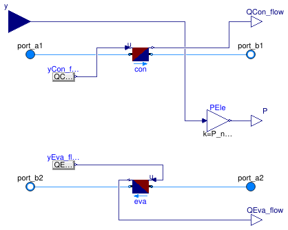
This is a model of a chiller whose coefficient of performance COP changes with temperatures in the same way as the Carnot efficiency changes. The input signal y is the control signal for the compressor.
Set use_eta_Carnot_nominal=true to specify directly
the Carnot effectiveness ηCarnot,0,
in which case the value of the parameter COP_nominal
will not affect the simulation.
If use_eta_Carnot_nominal=false, the model will use
the value of the parameter COP_nominal
together with the specified nominal temperatures
to compute the Carnot effectiveness as
ηCarnot,0 = COP0 ⁄ (Teva,0 ⁄ (Tcon,0 + Tapp,con,0 - (Teva,0-Tapp,eva,0))),
where Teva,0 is the evaporator temperature, Tcon,0 is the condenser temperature, Tapp,eva,0 is the evaporator approach temperature and Tapp,con,0 is the condenser approach temperature.
The COP is computed as the product
COP = ηCarnot,0 COPCarnot ηPL,
where COPCarnot is the Carnot efficiency and ηPL is the part load efficiency, expressed using a polynomial. This polynomial has the form
ηPL = a1 + a2 y + a3 y2 + ...,
where y ∈ [0, 1] is
the part load for cooling and the coefficients ai
are declared by the parameter a.
On the Dynamics tag, the model can be parametrized to compute a transient
or steady-state response.
The transient response of the model is computed using a first
order differential equation for the evaporator and condenser fluid volumes.
The chiller outlet temperatures are equal to the temperatures of these lumped volumes.
Typical use and important parameters
When using this component, make sure that the evaporator and the condenser have sufficient mass flow rate. Based on the mass flow rates, the compressor power, temperature difference and the efficiencies, the model computes how much heat will be added to the condenser and removed at the evaporator. If the mass flow rates are too small, very high temperature differences can result.
The evaporator heat flow rate QEva_flow_nominal is used to assign
the default value for the mass flow rates, which are used for the pressure drop
calculations.
It is also used to compute the part load efficiency.
Hence, make sure that QEva_flow_nominal is set to a reasonable value.
The maximum cooling capacity is set by the parameter QEva_flow_min,
which is by default set to negative infinity.
The coefficient of performance depends on the evaporator and condenser leaving temperature since otherwise the second law of thermodynamics may be violated.
Notes
For a similar model that can be used as a heat pump, see Buildings.Fluid.HeatPumps.Carnot_y.
Extends from Buildings.Fluid.Chillers.BaseClasses.PartialCarnot_y (Partial chiller model with performance curve adjusted based on Carnot efficiency).
Parameters
| Type | Name | Default | Description |
|---|---|---|---|
| replaceable package Medium1 | PartialMedium | Medium 1 in the component | |
| replaceable package Medium2 | PartialMedium | Medium 2 in the component | |
| Nominal condition | |||
| MassFlowRate | m1_flow_nominal | QCon_flow_nominal/cp1_defaul... | Nominal mass flow rate [kg/s] |
| MassFlowRate | m2_flow_nominal | QEva_flow_nominal/cp2_defaul... | Nominal mass flow rate [kg/s] |
| TemperatureDifference | dTEva_nominal | -10 | Temperature difference evaporator outlet-inlet [K] |
| TemperatureDifference | dTCon_nominal | 10 | Temperature difference condenser outlet-inlet [K] |
| Pressure | dp1_nominal | Pressure difference over condenser [Pa] | |
| Pressure | dp2_nominal | Pressure difference over evaporator [Pa] | |
| Power | P_nominal | Nominal compressor power (at y=1) [W] | |
| Efficiency | |||
| Boolean | use_eta_Carnot_nominal | true | Set to true to use Carnot effectiveness etaCarnot_nominal rather than COP_nominal |
| Real | etaCarnot_nominal | 0.3 | Carnot effectiveness (=COP/COP_Carnot) used during simulation if use_eta_Carnot_nominal = true [1] |
| Real | COP_nominal | etaCarnot_nominal*TUseAct_no... | Coefficient of performance at TEva_nominal and TCon_nominal, used during simulation if use_eta_Carnot_nominal = false [1] |
| Temperature | TCon_nominal | 303.15 | Condenser temperature used to compute COP_nominal if use_eta_Carnot_nominal=false [K] |
| Temperature | TEva_nominal | 278.15 | Evaporator temperature used to compute COP_nominal if use_eta_Carnot_nominal=false [K] |
| Real | a[:] | {1} | Coefficients for efficiency curve (need p(a=a, yPL=1)=1) |
| TemperatureDifference | TAppCon_nominal | if cp1_default < 1500 then 5... | Temperature difference between refrigerant and working fluid outlet in condenser [K] |
| TemperatureDifference | TAppEva_nominal | if cp2_default < 1500 then 5... | Temperature difference between refrigerant and working fluid outlet in evaporator [K] |
| Assumptions | |||
| Boolean | allowFlowReversal1 | true | = false to simplify equations, assuming, but not enforcing, no flow reversal for medium 1 |
| Boolean | allowFlowReversal2 | true | = false to simplify equations, assuming, but not enforcing, no flow reversal for medium 2 |
| Advanced | |||
| MassFlowRate | m1_flow_small | 1E-4*abs(m1_flow_nominal) | Small mass flow rate for regularization of zero flow [kg/s] |
| MassFlowRate | m2_flow_small | 1E-4*abs(m2_flow_nominal) | Small mass flow rate for regularization of zero flow [kg/s] |
| Diagnostics | |||
| Boolean | show_T | false | = true, if actual temperature at port is computed |
| Flow resistance | |||
| Condenser | |||
| Boolean | from_dp1 | false | = true, use m_flow = f(dp) else dp = f(m_flow) |
| Boolean | linearizeFlowResistance1 | false | = true, use linear relation between m_flow and dp for any flow rate |
| Real | deltaM1 | 0.1 | Fraction of nominal flow rate where flow transitions to laminar [1] |
| Evaporator | |||
| Boolean | from_dp2 | false | = true, use m_flow = f(dp) else dp = f(m_flow) |
| Boolean | linearizeFlowResistance2 | false | = true, use linear relation between m_flow and dp for any flow rate |
| Real | deltaM2 | 0.1 | Fraction of nominal flow rate where flow transitions to laminar [1] |
| Dynamics | |||
| Condenser | |||
| Time | tau1 | 60 | Time constant at nominal flow rate (used if energyDynamics1 <> Modelica.Fluid.Types.Dynamics.SteadyState) [s] |
| Temperature | T1_start | Medium1.T_default | Initial or guess value of set point [K] |
| Evaporator | |||
| Time | tau2 | 60 | Time constant at nominal flow rate (used if energyDynamics2 <> Modelica.Fluid.Types.Dynamics.SteadyState) [s] |
| Temperature | T2_start | Medium2.T_default | Initial or guess value of set point [K] |
| Evaporator and condenser | |||
| Dynamics | energyDynamics | Modelica.Fluid.Types.Dynamic... | Type of energy balance: dynamic (3 initialization options) or steady state |
Connectors
| Type | Name | Description |
|---|---|---|
| FluidPort_a | port_a1 | Fluid connector a1 (positive design flow direction is from port_a1 to port_b1) |
| FluidPort_b | port_b1 | Fluid connector b1 (positive design flow direction is from port_a1 to port_b1) |
| FluidPort_a | port_a2 | Fluid connector a2 (positive design flow direction is from port_a2 to port_b2) |
| FluidPort_b | port_b2 | Fluid connector b2 (positive design flow direction is from port_a2 to port_b2) |
| output RealOutput | QCon_flow | Actual heating heat flow rate added to fluid 1 [W] |
| output RealOutput | P | Electric power consumed by compressor [W] |
| output RealOutput | QEva_flow | Actual cooling heat flow rate removed from fluid 2 [W] |
| input RealInput | y | Part load ratio of compressor [1] |
Modelica definition
 Buildings.Fluid.Chillers.ElectricEIR
Electric chiller based on the DOE-2.1 model
Information
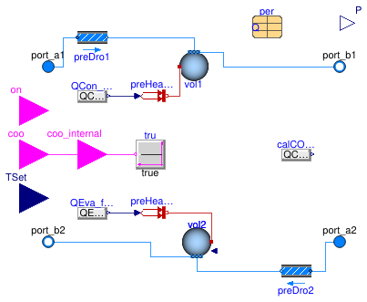
Model of an electric chiller, based on the DOE-2.1 chiller model and
the EnergyPlus chiller model Chiller:Electric:EIR.
This model uses three functions to predict capacity and power consumption:
| Function | Description | Formulation | |
|---|---|---|---|
ElectricEIR (this model) |
ElectricReformulatedEIR |
||
capFunT |
Adjusts cooling capacity for current fluid temperatures | Biquadratic on TConEnt and TEvaLvg |
Biquadratic on TConLvg and TEvaLvg |
EIRFunPLR |
Adjusts EIR for the current PLR | Quadratic on PLR | Bicubic on TConLvg and PLR |
EIRFunT |
Adjusts EIR for current fluid temperatures | Biquadratic on TConEnt and TEvaLvg |
Biquadratic on TConLvg and TEvaLvg |
These functions take the same form as documented in
EnergyPlus v22.1.0 Engineering Reference
section 14.3.9.2 (equations 14.231 through 14.233).
These curves are stored in the data record per and are available from
Buildings.Fluid.Chillers.Data.ElectricEIR.
How they are used to compute the adjusted capacity and compressor power
can be found in the documentation of
Buildings.Fluid.Chillers.BaseClasses.PartialElectric.
Additional performance curves can be developed using
two available techniques (Hydeman and Gillespie, 2002). The first technique is called the
Least-squares Linear Regression method and is used when sufficient performance data exist
to employ standard least-square linear regression techniques. The second technique is called
Reference Curve Method and is used when insufficient performance data exist to apply linear
regression techniques. A detailed description of both techniques can be found in
Hydeman and Gillespie (2002).
The model takes as an input the set point for the leaving chilled water temperature, which is met if the chiller has sufficient capacity. Thus, the model has a built-in, ideal temperature control. The model has three tests on the part load ratio and the cycling ratio:
-
The test
PLR1 =min(QEva_flow_set/QEva_flow_ava, per.PLRMax);
ensures that the chiller capacity does not exceed the chiller capacity specified by the parameterper.PLRMax. -
The test
CR = min(PLR1/per.PRLMin, 1.0);
computes a cycling ratio. This ratio expresses the fraction of time that a chiller would run if it were to cycle because its load is smaller than the minimal load at which it can operate. Note that this model continuously operates even if the part load ratio is below the minimum part load ratio. Its leaving evaporator and condenser temperature can therefore be considered as an average temperature between the modes where the compressor is off and on. -
The test
PLR2 = max(per.PLRMinUnl, PLR1);
computes the part load ratio of the compressor. The assumption is that for a part load ratio belowper.PLRMinUnl, the chiller uses hot gas bypass to reduce the capacity, while the compressor power draw does not change.
The electric power only contains the power for the compressor, but not any power for pumps or fans.
The model can be parametrized to compute a transient or steady-state response. The transient response of the chiller is computed using a first order differential equation for the evaporator and condenser fluid volumes. The chiller outlet temperatures are equal to the temperatures of these lumped volumes.
Optionally, the model can be configured to represent heat recovery chillers with
a switchover option by setting the parameter have_switchover to
true.
In that case an additional Boolean input connector coo is used.
The chiller is tracking a chilled water supply temperature setpoint at the
outlet of the evaporator barrel if coo is true.
Otherwise, if coo is false, the chiller is tracking
a hot water supply temperature setpoint at the outlet of the condenser barrel.
See
Buildings.Fluid.Chillers.Examples.ElectricEIR_HeatRecovery
for an example with a chiller operating in heating mode.
References
- Hydeman, M. and K.L. Gillespie. 2002. Tools and Techniques to Calibrate Electric Chiller Component Models. ASHRAE Transactions, AC-02-9-1.
- EnergyPlus v22.1.0 Engineering Reference
Extends from Buildings.Fluid.Chillers.BaseClasses.PartialElectric (Partial model for electric chiller based on the model in DOE-2, CoolTools and EnergyPlus).
Parameters
| Type | Name | Default | Description |
|---|---|---|---|
| replaceable package Medium1 | PartialMedium | Medium 1 in the component | |
| replaceable package Medium2 | PartialMedium | Medium 2 in the component | |
| MixingVolumeHeatPort | vol1 | vol1(final prescribedHeatFlo... | Volume for fluid 1 |
| Boolean | have_switchover | false | Set to true for heat recovery chiller with built-in switchover |
| Generic | per | Performance data | |
| Nominal condition | |||
| MassFlowRate | m1_flow_nominal | mCon_flow_nominal | Nominal mass flow rate [kg/s] |
| MassFlowRate | m2_flow_nominal | mEva_flow_nominal | Nominal mass flow rate [kg/s] |
| PressureDifference | dp1_nominal | Pressure difference [Pa] | |
| PressureDifference | dp2_nominal | Pressure difference [Pa] | |
| Initialization | |||
| Real | PLR1.start | 0 | Part load ratio [1] |
| Assumptions | |||
| Boolean | allowFlowReversal1 | true | = false to simplify equations, assuming, but not enforcing, no flow reversal for medium 1 |
| Boolean | allowFlowReversal2 | true | = false to simplify equations, assuming, but not enforcing, no flow reversal for medium 2 |
| Advanced | |||
| MassFlowRate | m1_flow_small | 1E-4*abs(m1_flow_nominal) | Small mass flow rate for regularization of zero flow [kg/s] |
| MassFlowRate | m2_flow_small | 1E-4*abs(m2_flow_nominal) | Small mass flow rate for regularization of zero flow [kg/s] |
| Diagnostics | |||
| Boolean | show_T | false | = true, if actual temperature at port is computed |
| Flow resistance | |||
| Medium 1 | |||
| Boolean | from_dp1 | false | = true, use m_flow = f(dp) else dp = f(m_flow) |
| Boolean | linearizeFlowResistance1 | false | = true, use linear relation between m_flow and dp for any flow rate |
| Real | deltaM1 | 0.1 | Fraction of nominal flow rate where flow transitions to laminar |
| Medium 2 | |||
| Boolean | from_dp2 | false | = true, use m_flow = f(dp) else dp = f(m_flow) |
| Boolean | linearizeFlowResistance2 | false | = true, use linear relation between m_flow and dp for any flow rate |
| Real | deltaM2 | 0.1 | Fraction of nominal flow rate where flow transitions to laminar |
| Dynamics | |||
| Nominal condition | |||
| Time | tau1 | 30 | Time constant at nominal flow [s] |
| Time | tau2 | 30 | Time constant at nominal flow [s] |
| Conservation equations | |||
| Dynamics | energyDynamics | Modelica.Fluid.Types.Dynamic... | Type of energy balance: dynamic (3 initialization options) or steady state |
| Initialization | |||
| Medium 1 | |||
| AbsolutePressure | p1_start | Medium1.p_default | Start value of pressure [Pa] |
| Temperature | T1_start | 273.15 + 25 | Start value of temperature [K] |
| MassFraction | X1_start[Medium1.nX] | Medium1.X_default | Start value of mass fractions m_i/m [kg/kg] |
| ExtraProperty | C1_start[Medium1.nC] | fill(0, Medium1.nC) | Start value of trace substances |
| ExtraProperty | C1_nominal[Medium1.nC] | fill(1E-2, Medium1.nC) | Nominal value of trace substances. (Set to typical order of magnitude.) |
| Medium 2 | |||
| AbsolutePressure | p2_start | Medium2.p_default | Start value of pressure [Pa] |
| Temperature | T2_start | 273.15 + 5 | Start value of temperature [K] |
| MassFraction | X2_start[Medium2.nX] | Medium2.X_default | Start value of mass fractions m_i/m [kg/kg] |
| ExtraProperty | C2_start[Medium2.nC] | fill(0, Medium2.nC) | Start value of trace substances |
| ExtraProperty | C2_nominal[Medium2.nC] | fill(1E-2, Medium2.nC) | Nominal value of trace substances. (Set to typical order of magnitude.) |
Connectors
| Type | Name | Description |
|---|---|---|
| FluidPort_a | port_a1 | Fluid connector a1 (positive design flow direction is from port_a1 to port_b1) |
| FluidPort_b | port_b1 | Fluid connector b1 (positive design flow direction is from port_a1 to port_b1) |
| FluidPort_a | port_a2 | Fluid connector a2 (positive design flow direction is from port_a2 to port_b2) |
| FluidPort_b | port_b2 | Fluid connector b2 (positive design flow direction is from port_a2 to port_b2) |
| input BooleanInput | on | Set to true to enable compressor, or false to disable compressor |
| input RealInput | TSet | Set point for leaving chilled water temperature (condenser water if have_switchover=true and coo=false) [K] |
| output RealOutput | P | Electric power consumed by compressor [W] |
| output RealOutput | COP_h | Coefficient of performance of heating [1] |
| input BooleanInput | coo | Switchover signal: true for cooling, false for heating |
Modelica definition
 Buildings.Fluid.Chillers.ElectricReformulatedEIR
Electric chiller based on the DOE-2.1 model, but with performance as a function of condenser leaving instead of entering temperature
Information
Model of an electric chiller, based on the model by
Hydeman et al. (2002) that has been developed in the CoolTools project
and that is implemented in EnergyPlus as the model
Chiller:Electric:ReformulatedEIR.
This empirical model is similar to
Buildings.Fluid.Chillers.ElectricEIR.
The difference is that to compute the performance, this model
uses the condenser leaving temperature instead of the entering temperature,
and it uses a bicubic polynomial to compute the part load performance.
This model uses three functions to predict capacity and power consumption:
| Function | Description | Formulation | |
|---|---|---|---|
ElectricEIR (this model) |
ElectricReformulatedEIR (this model) |
||
capFunT |
Adjusts cooling capacity for current fluid temperatures | Biquadratic on TConEnt and TEvaLvg |
Biquadratic on TConLvg and TEvaLvg |
EIRFunPLR |
Adjusts EIR for the current PLR | Quadratic on PLR | Bicubic on TConLvg and PLR |
EIRFunT |
Adjusts EIR for current fluid temperatures | Biquadratic on TConEnt and TEvaLvg |
Biquadratic on TConLvg and TEvaLvg |
These curves are stored in the data record per and are available from
Buildings.Fluid.Chillers.Data.ElectricReformulatedEIR.
How they are used to compute the adjusted capacity and compressor power
can be found in the documentation of
Buildings.Fluid.Chillers.BaseClasses.PartialElectric.
Additional performance curves can be developed using
two available techniques (Hydeman and Gillespie, 2002). The first technique is called the
Least-squares Linear Regression method and is used when sufficient performance data exist
to employ standard least-square linear regression techniques. The second technique is called
Reference Curve Method and is used when insufficient performance data exist to apply linear
regression techniques. A detailed description of both techniques can be found in
Hydeman and Gillespie (2002).
The model takes as an input the set point for the leaving chilled water temperature, which is met if the chiller has sufficient capacity. Thus, the model has a built-in, ideal temperature control. The model has three tests on the part load ratio and the cycling ratio:
-
The test
PLR1 =min(QEva_flow_set/QEva_flow_ava, per.PLRMax);
ensures that the chiller capacity does not exceed the chiller capacity specified by the parameterper.PLRMax. -
The test
CR = min(PLR1/per.PRLMin, 1.0);
computes a cycling ratio. This ratio expresses the fraction of time that a chiller would run if it were to cycle because its load is smaller than the minimal load at which it can operate. Note that this model continuously operates even if the part load ratio is below the minimum part load ratio. Its leaving evaporator and condenser temperature can therefore be considered as an average temperature between the modes where the compressor is off and on. -
The test
PLR2 = max(per.PLRMinUnl, PLR1);
computes the part load ratio of the compressor. The assumption is that for a part load ratio belowper.PLRMinUnl, the chiller uses hot gas bypass to reduce the capacity, while the compressor power draw does not change.
The electric power only contains the power for the compressor, but not any power for pumps or fans.
The model can be parametrized to compute a transient or steady-state response. The transient response of the chiller is computed using a first order differential equation for the evaporator and condenser fluid volumes. The chiller outlet temperatures are equal to the temperatures of these lumped volumes.
Optionally, the model can be configured to represent heat recovery chillers with
a switchover option by setting the parameter have_switchover to
true.
In that case an additional Boolean input connector coo is used.
The chiller is tracking a chilled water supply temperature setpoint at the
outlet of the evaporator barrel if coo is true.
Otherwise, if coo is false, the chiller is tracking
a hot water supply temperature setpoint at the outlet of the condenser barrel.
See
Buildings.Fluid.Chillers.Examples.ElectricEIR_HeatRecovery
for an example with a chiller operating in heating mode.
References
- Hydeman, M., N. Webb, P. Sreedharan, and S. Blanc. 2002. Development and Testing of a Reformulated Regression-Based Electric Chiller Model. ASHRAE Transactions, HI-02-18-2.
- Hydeman, M. and K.L. Gillespie. 2002. Tools and Techniques to Calibrate Electric Chiller Component Models. ASHRAE Transactions, AC-02-9-1.
Extends from Buildings.Fluid.Chillers.BaseClasses.PartialElectric (Partial model for electric chiller based on the model in DOE-2, CoolTools and EnergyPlus).
Parameters
| Type | Name | Default | Description |
|---|---|---|---|
| replaceable package Medium1 | PartialMedium | Medium 1 in the component | |
| replaceable package Medium2 | PartialMedium | Medium 2 in the component | |
| MixingVolumeHeatPort | vol1 | vol1(final prescribedHeatFlo... | Volume for fluid 1 |
| Boolean | have_switchover | false | Set to true for heat recovery chiller with built-in switchover |
| Generic | per | Performance data | |
| Nominal condition | |||
| MassFlowRate | m1_flow_nominal | mCon_flow_nominal | Nominal mass flow rate [kg/s] |
| MassFlowRate | m2_flow_nominal | mEva_flow_nominal | Nominal mass flow rate [kg/s] |
| PressureDifference | dp1_nominal | Pressure difference [Pa] | |
| PressureDifference | dp2_nominal | Pressure difference [Pa] | |
| Initialization | |||
| Real | PLR1.start | 0 | Part load ratio [1] |
| Assumptions | |||
| Boolean | allowFlowReversal1 | true | = false to simplify equations, assuming, but not enforcing, no flow reversal for medium 1 |
| Boolean | allowFlowReversal2 | true | = false to simplify equations, assuming, but not enforcing, no flow reversal for medium 2 |
| Advanced | |||
| MassFlowRate | m1_flow_small | 1E-4*abs(m1_flow_nominal) | Small mass flow rate for regularization of zero flow [kg/s] |
| MassFlowRate | m2_flow_small | 1E-4*abs(m2_flow_nominal) | Small mass flow rate for regularization of zero flow [kg/s] |
| Diagnostics | |||
| Boolean | show_T | false | = true, if actual temperature at port is computed |
| Flow resistance | |||
| Medium 1 | |||
| Boolean | from_dp1 | false | = true, use m_flow = f(dp) else dp = f(m_flow) |
| Boolean | linearizeFlowResistance1 | false | = true, use linear relation between m_flow and dp for any flow rate |
| Real | deltaM1 | 0.1 | Fraction of nominal flow rate where flow transitions to laminar |
| Medium 2 | |||
| Boolean | from_dp2 | false | = true, use m_flow = f(dp) else dp = f(m_flow) |
| Boolean | linearizeFlowResistance2 | false | = true, use linear relation between m_flow and dp for any flow rate |
| Real | deltaM2 | 0.1 | Fraction of nominal flow rate where flow transitions to laminar |
| Dynamics | |||
| Nominal condition | |||
| Time | tau1 | 30 | Time constant at nominal flow [s] |
| Time | tau2 | 30 | Time constant at nominal flow [s] |
| Conservation equations | |||
| Dynamics | energyDynamics | Modelica.Fluid.Types.Dynamic... | Type of energy balance: dynamic (3 initialization options) or steady state |
| Initialization | |||
| Medium 1 | |||
| AbsolutePressure | p1_start | Medium1.p_default | Start value of pressure [Pa] |
| Temperature | T1_start | 273.15 + 25 | Start value of temperature [K] |
| MassFraction | X1_start[Medium1.nX] | Medium1.X_default | Start value of mass fractions m_i/m [kg/kg] |
| ExtraProperty | C1_start[Medium1.nC] | fill(0, Medium1.nC) | Start value of trace substances |
| ExtraProperty | C1_nominal[Medium1.nC] | fill(1E-2, Medium1.nC) | Nominal value of trace substances. (Set to typical order of magnitude.) |
| Medium 2 | |||
| AbsolutePressure | p2_start | Medium2.p_default | Start value of pressure [Pa] |
| Temperature | T2_start | 273.15 + 5 | Start value of temperature [K] |
| MassFraction | X2_start[Medium2.nX] | Medium2.X_default | Start value of mass fractions m_i/m [kg/kg] |
| ExtraProperty | C2_start[Medium2.nC] | fill(0, Medium2.nC) | Start value of trace substances |
| ExtraProperty | C2_nominal[Medium2.nC] | fill(1E-2, Medium2.nC) | Nominal value of trace substances. (Set to typical order of magnitude.) |
Connectors
| Type | Name | Description |
|---|---|---|
| FluidPort_a | port_a1 | Fluid connector a1 (positive design flow direction is from port_a1 to port_b1) |
| FluidPort_b | port_b1 | Fluid connector b1 (positive design flow direction is from port_a1 to port_b1) |
| FluidPort_a | port_a2 | Fluid connector a2 (positive design flow direction is from port_a2 to port_b2) |
| FluidPort_b | port_b2 | Fluid connector b2 (positive design flow direction is from port_a2 to port_b2) |
| input BooleanInput | on | Set to true to enable compressor, or false to disable compressor |
| input RealInput | TSet | Set point for leaving chilled water temperature (condenser water if have_switchover=true and coo=false) [K] |
| output RealOutput | P | Electric power consumed by compressor [W] |
| output RealOutput | COP_h | Coefficient of performance of heating [1] |
| input BooleanInput | coo | Switchover signal: true for cooling, false for heating |