Examples

Simulating a model with two different parameter values

This module provides an example that illustrates the use of the python to run a Modelica simulation.

The module buildingspy.simulate that can be used to automate running simulations. For example, to translate and simulate the model Buildings.Fluid.SolarCollectors.Examples.FlatPlateWithTank from the Modelica Buildings Library, release 9.1.0, with different sizes for the water tank, use the following commands:

#!/usr/bin/env python
# -*- coding: utf-8 -*-
#
from multiprocessing import Pool

from buildingspy.simulate.Dymola import Simulator


# Function to set common parameters and to run the simulation
def simulateCase(s):
    """ Set common parameters and run a simulation.

    :param s: A simulator object.

    """
    s.setStopTime(24 * 3600)
    # Kill the process if it does not finish in 1 minute
    s.setTimeOut(60)
    s.printModelAndTime()
    s.simulate()


def main():
    """ Main method that configures and runs all simulations
    """
    import shutil

    # Build list of cases to run
    li = []
    # First model, from Modelica Buildings Library, v9.1.0
    model = 'Buildings.Fluid.SolarCollectors.Examples.FlatPlateWithTank'
    s = Simulator(model, outputDirectory='case1')
    s.addParameters({'tan.VTan': 1.5})
    li.append(s)
    # second model
    s = Simulator(model, outputDirectory='case2')
    s.addParameters({'tan.VTan': 2})
    li.append(s)

    # Run all cases in parallel
    po = Pool()
    po.map(simulateCase, li)
    po.close()
    po.join()

    # Clean up
    shutil.rmtree('case1')
    shutil.rmtree('case2')


# Main function
if __name__ == '__main__':
    main()

This will run the two test cases and store the results in the directories case1 and case2. To use Optimica instead of Dymola, replace in the above script Dymola with Optimica.

Plotting of Time Series

This module provides an example that illustrates the use of the python to plot results from a Dymola simulation. See also the class buildingspy.io.postprocess.Plotter for more advanced plotting.

The file plotResult.py illustrates how to plot results from a Dymola output file. To run the example, proceed as follows:

1. Open a terminal or dos-shell.

2. Set the PYTHONPATH environment variables to the directory that contains `buildingspy` as a subdirectory, such as

   cd buildingspy/examples/dymola
   export PYTHONPATH=${PYTHONPATH}:../../..
   

3. Type

   python plotResult.py
   

This will execute the script plotResult.py, which contains the following instructions:

#!/usr/bin/env python
# -*- coding: utf-8 -*-
#

def main():
    """ Main method that plots the results
    """
    import os

    import matplotlib
    matplotlib.use('Agg')
    import matplotlib.pyplot as plt

    from buildingspy.io.outputfile import Reader

    # Optionally, change fonts to use LaTeX fonts
    # from matplotlib import rc
    # rc('text', usetex=True)
    # rc('font', family='serif')

    # Read results
    ofr1 = Reader(os.path.join("buildingspy", "examples", "dymola",
                               "case1", "FlatPlateWithTank.mat"), "dymola")
    ofr2 = Reader(os.path.join("buildingspy", "examples", "dymola",
                               "case2", "FlatPlateWithTank.mat"), "dymola")
    (time1, TIn1) = ofr1.values("TIn.T")
    (time1, TOut1) = ofr1.values("TOut.T")
    (time2, TIn2) = ofr2.values("TIn.T")
    (time2, TOut2) = ofr2.values("TOut.T")

    # Plot figure
    fig = plt.figure()
    ax = fig.add_subplot(111)

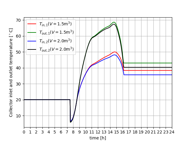
    ax.plot(time1 / 3600, TIn1 - 273.15, 'r', label='$T_{in,1}(V=1.5 \\mathrm{m^3})$')
    ax.plot(time1 / 3600, TOut1 - 273.15, 'g', label='$T_{out,1}(V=1.5 \\mathrm{m^3})$')
    ax.plot(time2 / 3600, TIn2 - 273.15, 'b', label='$T_{in,2}(V=2.0 \\mathrm{m^3})$')
    ax.plot(time2 / 3600, TOut2 - 273.15, 'k', label='$T_{out,2}(V=2.0 \\mathrm{m^3})$')

    ax.set_xlabel('time [h]')
    ax.set_ylabel(r'Collector inlet and outlet temperature [$^\circ$C]')
    ax.set_xticks(list(range(25)))
    ax.set_xlim([0, 24])
    ax.legend()
    ax.grid(True)

    # Save figure to file
    plt.savefig('plot.pdf')
    plt.savefig('plot.png')

    # To show the plot on the screen, uncomment the line below
    # plt.show()


# Main function
if __name__ == '__main__':
    main()

The script generates the following plot: