Buildings.Fluid.HeatExchangers.RadiantSlabs.UsersGuide

User's Guide

Information

Heat transfer through the slab

The figure below shows the thermal resistance network of the model for an example in which the pipes are embedded in the concrete slab, and the layers below the pipes are insulation and reinforced concrete.

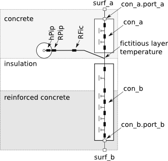
The construction con_a computes transient heat conduction between the surface heat port surf_a and the plane that contains the pipes, with the heat port con_a.port_a connecting to surf_a. Similarly, the construction con_b is between the plane that contains the pipes and the surface heat port sur_b, with the heat port con_b.port_b connecting to surf_b. The temperature of the plane that contains the pipes is computes using a fictitious resistance RFic, which is computed by Buildings.Fluid.HeatExchangers.RadiantSlabs.BaseClasses.Functions.AverageResistance. There is also a resistance for the pipe wall RPip and a convective heat transfer coefficient between the fluid and the pipe inside wall. The convective heat transfer coefficient is a function of the mass flow rate and is computed in Buildings.Fluid.HeatExchangers.RadiantSlabs.BaseClasses.PipeToSlabConductance.

Material layers

The material layers are declared by the parameter layers, which is an instance of Buildings.HeatTransfer.Data.OpaqueConstructions. The first layer of this material is the one at the heat port surf_a, and the last layer is at the heat port surf_b. The parameter iLayPip must be set to the number of the interface in which the pipes are located. For example, consider the following floor slab.

Then, the construction definition is

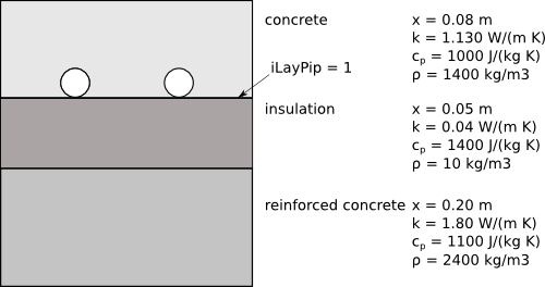
  Buildings.HeatTransfer.Data.OpaqueConstructions.Generic layers(
        nLay=3,
        material={
          Buildings.HeatTransfer.Data.Solids.Generic(
            x=0.08,
            k=1.13,
            c=1000,
            d=1400,
            nSta=5),
          Buildings.HeatTransfer.Data.Solids.Generic(
            x=0.05,
            k=0.04,
            c=1400,
            d=10),
          Buildings.HeatTransfer.Data.Solids.Generic(
            x=0.2,
            k=1.8,
            c=1100,
            d=2400)}) "Material definition for floor construction";

Note that we set nSta=5 in the first material layer. In this example, this material layer is the concrete layer in which the pipes are embedded. By setting nSta=5 the simulation is forced to be done with five state variables in this layer. The default setting would have led to only one state variable in this layer.

Since the pipes are at the interface of the concrete and the insulation, we set iLayPip=1.

Discretization along the flow path

If the parameter heatTransfer=EpsilonNTU, then the heat transfer between the fluid and the fictitious layer temperature is computed using an ε-NTU model. If heatTransfer=FiniteDifference, then the pipe and the slab is discretized along the water flow direction and a finite difference model is used to compute the heat transfer. The parameter nSeg determines how many times the resistance network is instantiated along the flow path. However, all instances connect to the same surface temperature heat ports surf_a and surf_b.

The default value for is nSeg=1 if heatTransfer=EpsilonNTU and nSeg=5 if heatTransfer=FiniteDifference. For a typical building simulation, we recommend to use the default settings of heatTransfer=EpsilonNTU and nSeg=1, as these lead to fastest computing time. However, for feedback control design in which the outlet temperature of the slab is used, one may want to use heatTransfer=FiniteDifference and nSeg=5. This will cause the model to use 5 parallel segments in which heat is conducted between the control volume of the pipe fluid and the surfaces of the slab. 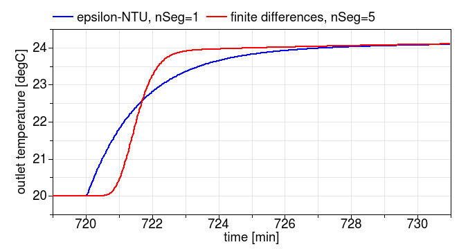While the heat flow rate at the surface does not change noticeably between these two configurations, the dynamics of the water outlet temperature from the slab is significantly different. The figure below shows the water outlet temperature response to a step change in the volume flow rate at t=720 minutes. One can see that if heatTransfer=EpsilonNTU and nSeg=1, the response looks like a first order response (because nSeg=1), while with heatTransfer=FiniteDifference and nSeg=5, the response is higher order. This figure was generated using Buildings.Fluid.HeatExchangers.RadiantSlabs.Examples.StepResponseFiniteDifference and Buildings.Fluid.HeatExchangers.RadiantSlabs.Examples.StepResponseEpsilonNTU\.

Initialization

The initialization of the fluid in the pipes and of the slab temperature are independent of each other.

To initialize the medium, the same mechanism is used as for any other fluid volume, such as Buildings.Fluid.MixingVolumes.MixingVolume. Specifically, the parameters energyDynamics and massDynamics on the Dynamics tab are used. Depending on the values of these parameters, the medium is initialized using the values p_start, T_start, X_start and C_start, provided that the medium model contains species concentrations X and trace substances C.

To initialize the construction temperatures, the parameters steadyStateInitial, T_a_start, T_b_start and T_c_start are used. By default, T_c_start is set to the temperature that leads to steady-state heat transfer between the surfaces surf_a and surf_b, whose temperatures are both set to T_a_start and T_b_start.

The parameter pipe, which is an instance of the record Buildings.Fluid.Data.Pipes, defines the pipe material and geometry. The parameter disPip declares the spacing between the pipes and the parameter length, with default length=A/disPip where A is the slab surface area, declares the whole length of the pipe circuit.

The parameter sysTyp is used to select the equation that is used to compute the average temperature in the plane of the pipes. It needs to be set to the following values:

sysTyp	System type
BaseClasses.Types.SystemType.Floor	Radiant heating or cooling systems with pipes embedded in the concrete slab above the thermal insulation.
BaseClasses.Types.SystemType.Ceiling_Wall_or_Capillary	Radiant heating or cooling systems with pipes embedded in the concrete slab in the ceiling, or radiant wall systems. Radiant heating and cooling systems with capillary heat exchanger at the construction surface.

Limitations

The analogy with a three-resistance network and the corresponding equation for Rx is based on a steady-state heat transfer analysis. Therefore, it is only valid during steady-state. For a fully dynamic model, a three-dimensional finite element method for the radiant slab would need to be implemented.

Implementation

To separate the material declaration layers into layers between the pipes and heat port surf_a, and between the pipes and surf_b, the vector layers.material[nLay] is partitioned into layers.material[1:iLayPip] and layers.material[iLayPip+1:nLay]. The respective partitions are then assigned to the models for heat conduction between the plane with the pipes and the construction surfaces, con_a and con_b.

Extends from Modelica.Icons.Information (Icon for general information packages).

---